
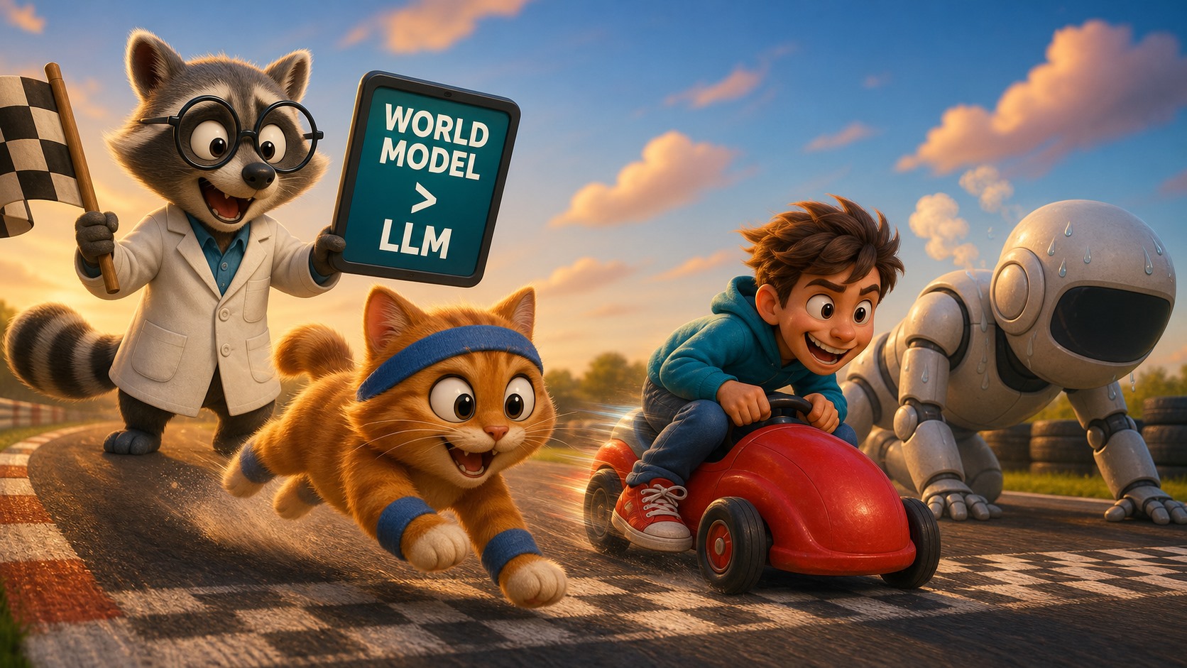
One of the fathers of deep learning, Yann LeCun, has been telling everyone for several years that autoregressive large language models are a dead end on the road to human-level intelligence. Not merely "an imperfect road", but specifically a dead end; in LeCun's view, scaling up next-token prediction alone will never get us to a real understanding of the world. In this era of universal excitement about LLMs, this sounds quite heretical. LeCun does of course see that, on their way into this dead end, language models manage to, say, disprove Erdős conjectures, but that doesn't convince him.
His favorite argument is that a cat models the physics of the surrounding world better than any LLM, and that a teenager learns to drive in about twenty hours of practice, with no synthetic RL environment, because they already have a model of the world in which they can "roll forward" the consequences of turning the wheel without actually flying into a ditch.
In this post I want to tell you what LeCun bets on instead of language models, and along the way to give a general introduction to the topic, tracing what is essentially one and the same idea across thirty years of its history, from Siamese networks in 1993 to modern world models.
There will be plenty of technical detail, but I'll try to keep the intuition visible at every step, so that the individual pieces add up to a single, hopefully coherent picture. The post will be long and fairly theoretical, in the spirit of our previous posts on the thermodynamics of training and TurboQuant. On the plus side, along the way we'll discuss a lot of different self-supervised learning methods, because JEPA is best understood not as one particular invention of 2022, but as the point where metric learning, contrastive learning, masked modeling, and world models all converge.
Let me point you to a couple of other expositions right away: the YouTube channel Welch Labs put out a two-part explainer called "Yann LeCun's $1B Bet Against LLMs" (part 1, part 2), which LeCun himself reposted, calling it an "excellent tutorial video". There's also a detailed blog post by Rohit Bandaru called "Deep Dive into Yann LeCun's JEPA", a great post, but you and I will take a broader view and go to the primary sources.
The acronym JEPA stands for Joint-Embedding Predictive Architecture. And the main idea in all of this can be summarized as follows:
Learning happens by predicting the representations (extracted abstract meaning) of what you don't see, rather than by prediing pixels or tokens. Good abstraction here is not an approximation but the whole point: a sensibly designed system should be able to throw away whatever is impossible or pointless to predict.
This sounds quite philosophical, and in the 2022 manifesto (LeCun, 2022) it is indeed presented rather abstractly. But the same idea appeared thirty years before the acronym JEPA, and soon after the position paper, variants of these models started showing up that solve some very practical tasks quite well. In this post we'll walk through that whole long road.
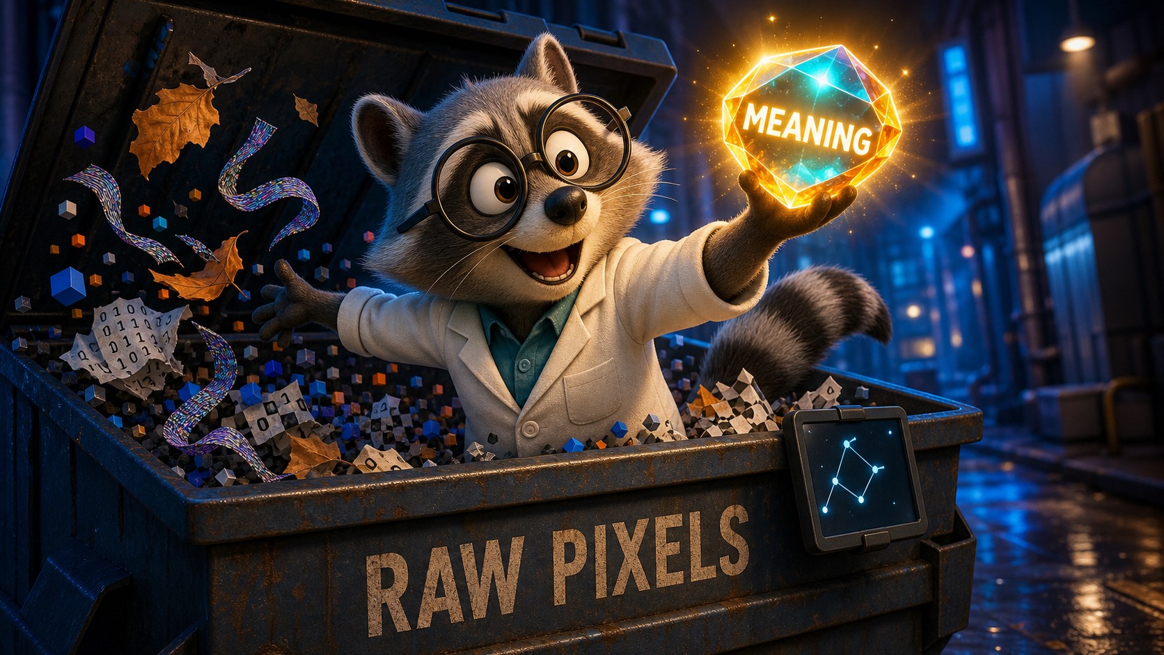
Before we plunge into the history, let us pin down the core idea in a more practically useful form. One thought recurs throughout this 30+-year history:
Take two views of the same little piece of the world, run each through a (possibly shared) encoder, and shape the geometry of the two resulting vectors relative to each other.
What changes from era to era are relatively secondary things:
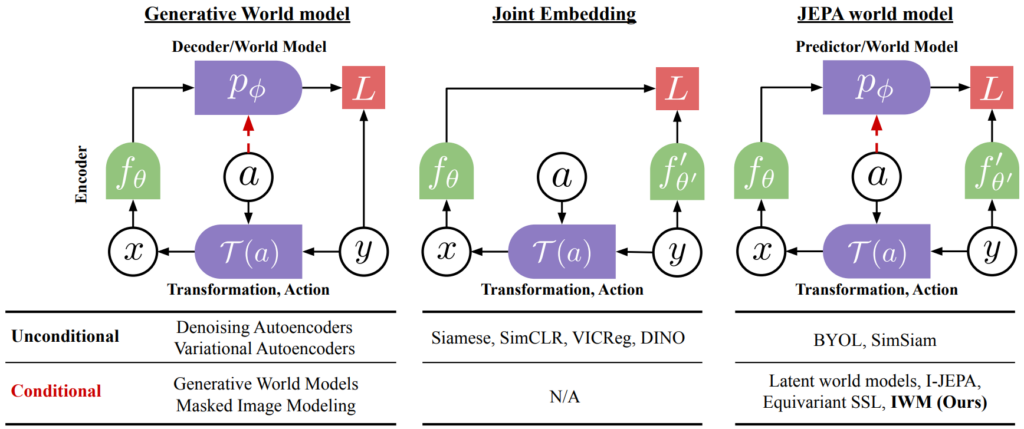
In the terminology of LeCun and his team, it's customary to distinguish three families of architectures; this split is best drawn in the very first figure of the I-JEPA paper (Assran et al., 2023):

The difference between JEA and JEPA is subtle but fundamental: JEA requires x and y to be essentially interchangeable, hence the invariance to augmentations, whereas JEPA lets x and y carry different information. The context and the target need not be the same thing, but there is a relationship between them, and it's precisely this relationship that the predictor has to learn.
And here's the promised running example, a single "equation" that will evolve throughout the text. At each step we'll ask ourselves one and the same question, with only the phrasing changing slightly:
And here is the timeline of the whole road; it has five parallel threads of self-supervised learning, each running from left to right and eventually converging on the 2022 JEPA manifesto.
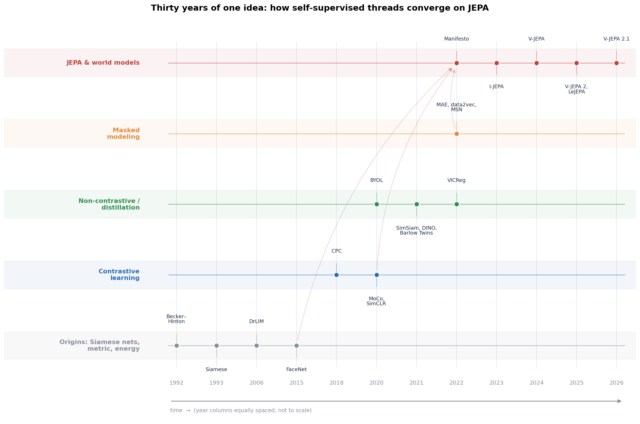
Now let us go through this timeline slowly, from the very beginning.
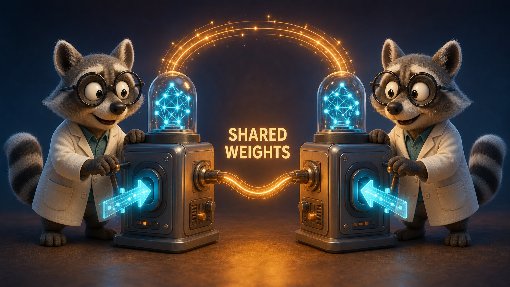
The history is usually started in 1993, but a year earlier, in 1992, Suzanna Becker and Geoffrey Hinton published a paper in Nature about a self-organizing network that discovers surfaces in random-dot stereograms (Becker, Hinton, 1992). It worked like this: two modules of the network look at *neighboring* patches of an image and learn to maximize the mutual information between their outputs, on the assumption that neighboring patches have a common hidden cause (the depth of a surface).
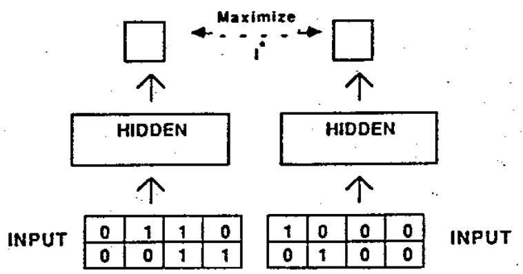
Structurally, this is already a clear forerunner of everything that follows: two encoders, a shared hidden target, learning through agreement. And the idea that good features are features cleansed of redundancy is older still: it goes back to the redundancy reduction principle of the neurophysiologist Horace Barlow (Barlow, 1961), and in neural network form it was formulated by that very same Schmidhuber as predictability minimization (Schmidhuber, 1992), where feature detectors compete with predictors that try to predict them from one another. We'll meet Barlow again below, when thirty years later a method called Barlow Twins is named precisely in his honor.
The actual history of Siamese networks begins with the paper "Signature Verification using a 'Siamese' Time Delay Neural Network" (Bromley et al., 1993; the authors, incidentally, included Yann LeCun himself). The paper solved a very practical task—verifying that a signature on a check is genuine, i.e. comparing a given signature with a real reference sample—but the idea that grew out of it proved to reach much further.
They took two identical subnetworks with shared weights (hence the name "Siamese"), each of which encodes one of the signatures into a feature vector, and then measured the distance between these vectors:
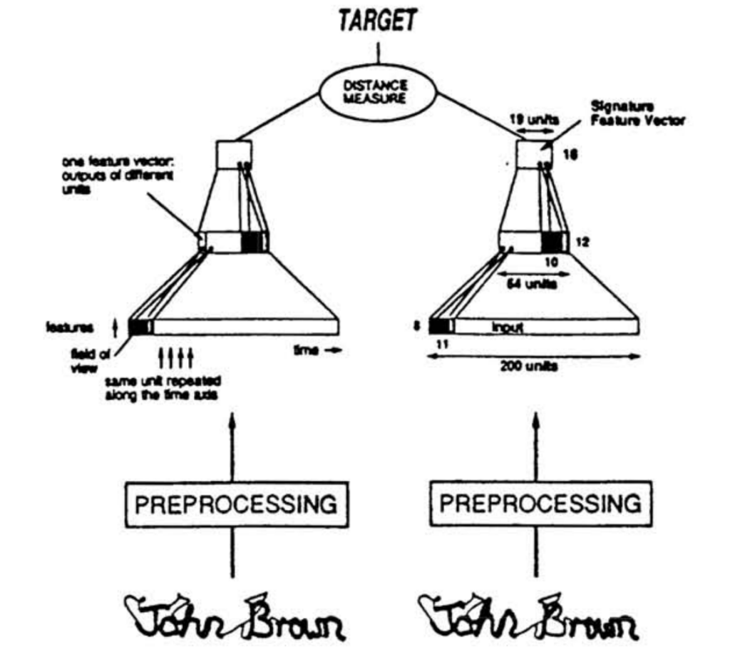
The idea, naturally, is to then treat a small distance as confirmation of authenticity and a large one as a forgery. The key, and at the time far from obvious, thing here is weight tying: both branches have the same weights, i.e. they produce the same geometry at the output. We stop training a classifier ("this is John Smith's signature") and start training the geometry of the feature space. This is the seed from which everything else grew.
The idea wasn't exactly forgotten, but it went undeveloped for a good decade. Only in the mid-2000s was it revived and generalized by, again, LeCun's group. Two papers that landed at CVPR back then turned the "Siamese trick" into a general principle of discriminative metric learning.
First came "Learning a Similarity Metric Discriminatively" (Chopra, Hadsell, LeCun, 2005) on face verification, built on exactly the same Siamese idea:
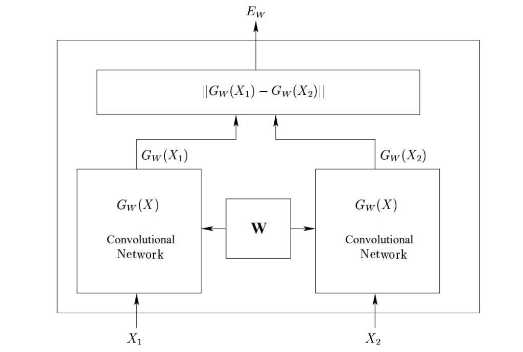
And then came one of the underappreciated classics: "Dimensionality Reduction by Learning an Invariant Mapping" (DrLIM; Hadsell, Chopra, LeCun, 2006). It's there that the contrastive loss function appears in its canonical form. Let a pair of objects carry a label Y (0 = "similar", 1 = "dissimilar"), and let $D_W$ be the distance between their embeddings; then
![\[\mathcal{L}(W) = (1-Y)\,\tfrac12\, D_W^2 \;+\; Y\,\tfrac12\,\big(\max(0,\; m - D_W)\big)^2.\]](https://cdn.prod.website-files.com/677e6981f4fde5d98559a350/6a579c07df275a431021569f_6a5791f330354a60de858bf8_6a4fad643eaf798e5ea82803_quicklatex.com-830bcf6f3cae0c1247aeea6a28f5d017_l3.svg)
The first term here works on similar pairs and "pulls" them towards each other. The second works on dissimilar ones, pushing them apart up to some margin value m; beyond the margin there's no need to push further, and the penalty goes to zero. The authors, by the way, explained all this in the language of mechanics: similar pairs are connected by springs that pull them together, and dissimilar ones by repulsive springs that stop acting at distance m; and in the end the whole construction should relax to equilibrium, like a physical system.
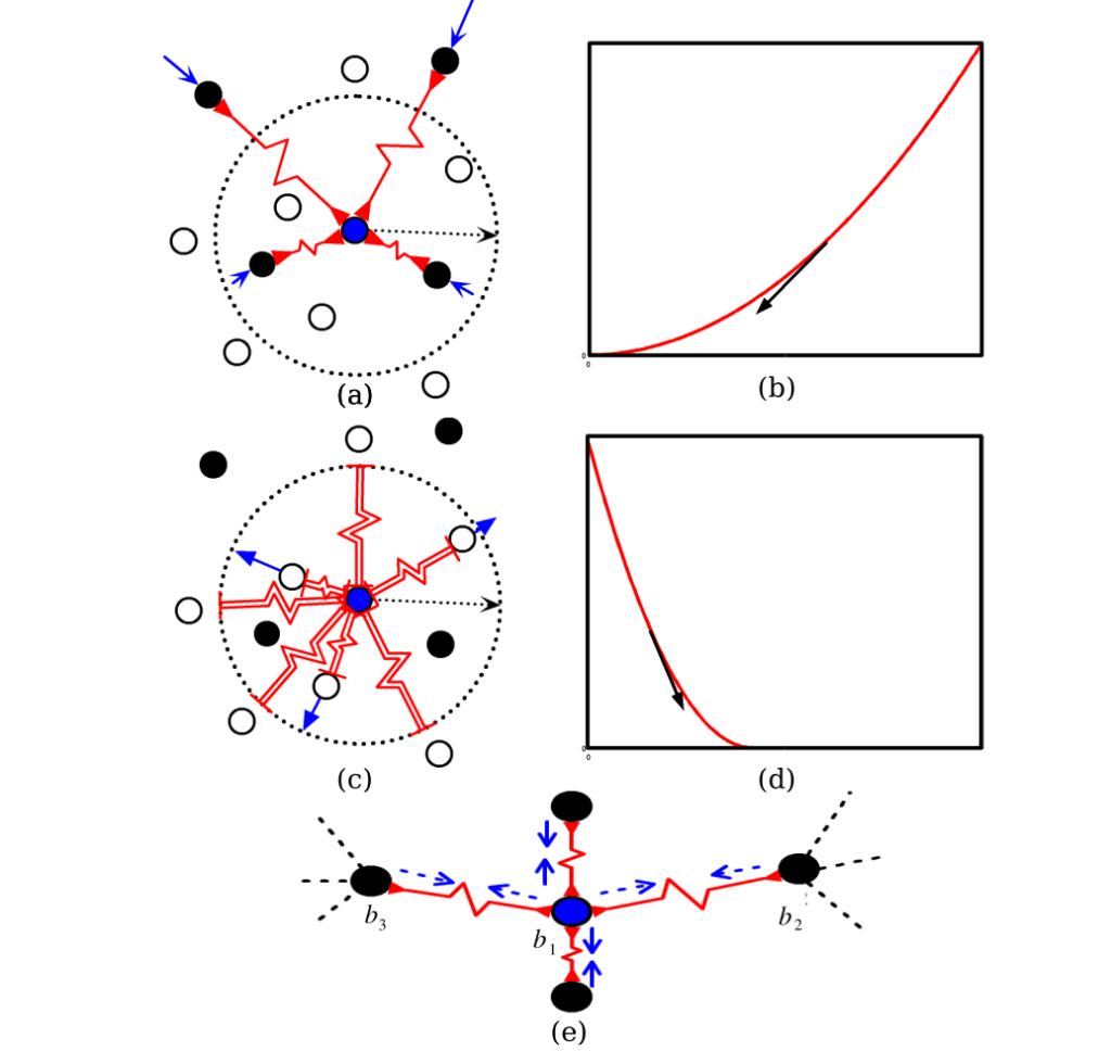
Here, incidentally, is where the collapse problem is first posed and solved. If you remove the second term, the network is left with one trivial solution: map absolutely everything to one and the same point. And if you add the term but with no margin, another one appears: keep dragging the embeddings of dissimilar objects apart to infinity. The margin m is there precisely so that neither of these happens.
The mature, well-known incarnation of this line was FaceNet (Schroff et al., 2015) with its triplet loss function: take an anchor a, a positive p (the same person), and a negative n (a different person), and require the anchor to be closer to the positive than to the negative by some margin α:
![\[|f(a)-f(p)|^2 + \alpha \;\le\; |f(a)-f(n)|^2.\]](https://cdn.prod.website-files.com/677e6981f4fde5d98559a350/6a579c07df275a4310215688_6a5791f230354a60de858be1_6a4fade351714e45ecc02236_quicklatex.com-643b522d13f3a8efc15abdbe60a0af2e_l3.svg)
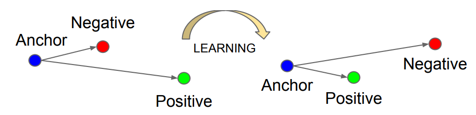
FaceNet is not an ancestor of JEPA in the narrow technical sense, but its historical role is large: it's the one that got everyone used to the idea that a model's output can be not a vector of class probabilities but a *reusable geometry of embeddings*. On top of that, FaceNet genuinely worked wonderfully and spawned an entire face-recognition industry that simply couldn't have existed before.
Finally, there's one more line in early deep learning without which the picture would be incomplete: energy-based learning. In the important position paper "A Tutorial on Energy-Based Learning" (LeCun et al., 2006), learning is described as shaping an energy function F(x,y): compatible configurations (x,y) should be assigned low energy, and incompatible ones high energy. And here a "configuration" no longer necessarily means similar objects; it can involve objects of quite different nature that simply correspond to each other one way or another:
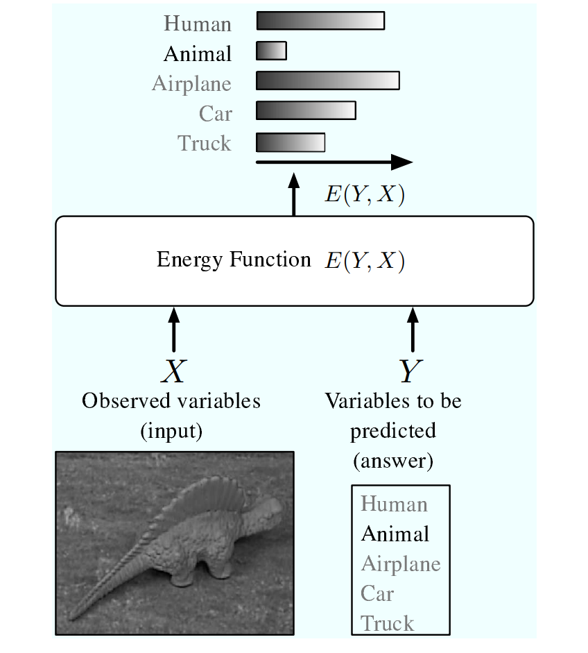
This view is, of course, older: it goes back to Hopfield networks (Hopfield, 1982) and Boltzmann machines (Ackley, Hinton, Sejnowski, 1985), and a good modern introduction to energy-based models with latent variables can be found in Dawid, LeCun (2023):
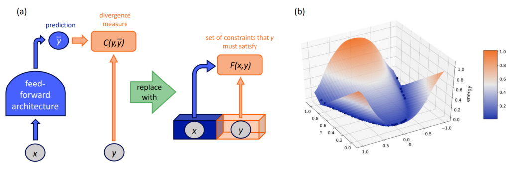
The contrastive loss from DrLIM turns out to be a special case: it pulls energy down on similar pairs and pushes it up on dissimilar ones.
The main trouble with energy-based models is that they look almost probabilistic, but making them actually probabilistic is hard. To turn energy into a probability, you have to divide it by a normalizing constant

Here Z has to be a sum over all conceivable configurations, which in high dimensions is simply impossible to compute. The essence of energy-based methods is to somehow sculpt the energy landscape you want without ever touching Z.
This energy-based lens will reappear below, because in the 2022 manifesto JEPA is formulated precisely as an energy-based model with a latent variable. For now, let's keep in mind one simple thought: contrastive, non-contrastive, and JEPA methods are not three completely different approaches, but three answers to one and the same question: how to raise the energy where there is no data, without computing that intractable normalizing constant.

Before going further, it's worth asking: why learn without labels at all? The answer is plain and prosaic: labeled data is expensive, while unlabeled data is practically infinite. But LeCun also has his famous gastronomic metaphor for this answer, "LeCun's cake" from NIPS 2016:
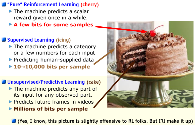
If intelligence is a cake, then self-supervised learning is the sponge itself, supervised learning is the icing, and reinforcement learning is the cherry on top. Almost all of the "mass" of what a human or animal learns comes from passively absorbing the structure of the world, and only a thin layer comes from direct instructions and rewards. Over the years LeCun has tweaked the recipe a few times (in the original version above the sponge was called unsupervised, then it became self-supervised), but the proportions haven't changed.
And in general the answer to "how do we learn without labels" looks quite natural: let's invent a task for which the labels come for free from the data itself, and hope that solving it forces the network to learn something useful. This is exactly how, for instance, the well-known language models learn everything under the sun just by predicting the next token.
Such tasks are called pretext tasks, and in image processing there were a great many of them. Exemplar-CNN (Dosovitskiy et al., 2014) declared each image its own separate class. Doersch et al. (2015) proposed, given two patches of one image, to guess their relative arrangement ("eye above nose").
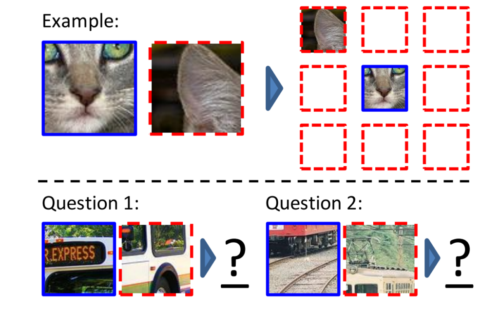
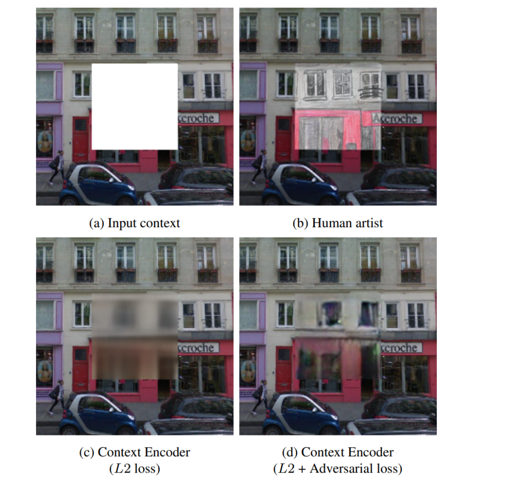
Then came assembling a jigsaw puzzle from shuffled pieces (Noroozi, Favaro, 2016), colorizing black-and-white photos (Zhang et al., 2016), and, most importantly, inpainting, asking the model to paint in a cut-out middle of a picture (Pathak et al., 2016); this is a direct ancestor of masked modeling:
There were also thoroughly minimalist tasks like RotNet (Gidaris et al., 2018): let's rotate the picture by 0, 90, 180, or 270 degrees and ask the network to guess by how much. It sounds utterly trivial, yet it worked surprisingly well: to figure out which way is up on a dog, you have to understand pretty well what a dog looks like.
There's one instructive story from this era, connected more to my perennial topic of AI Safety, or more precisely to the goodharting effect. Neural networks solved pretext tasks with enthusiasm, but not always by the method the authors had in mind.
For example, in the patch-arrangement task (Doersch et al., 2015) the network learned to cheat via chromatic aberration of the lens: in real photos the color channels are slightly shifted relative to each other radially from the center of the frame, and from that shift you can determine a patch's absolute position in the frame without looking at its content at all. The authors had to specifically break this leakage channel with color preprocessing.
In the end it turned out that a hand-crafted task will be solved by the cheapest available means, and no one guarantees that this means requires "understanding" or building a "model of the world". A systematic check (Kolesnikov et al., 2019) confirmed that pretext tasks are brittle and strongly depend on the architecture.
Meanwhile, in NLP a far more general loss function suited to this case had essentially already been found. Word2vec (Mikolov et al., 2013) trained word embeddings by predicting a word from its context, and its negative sampling is a simplified version of noise-contrastive estimation, NCE (Gutmann, Hyvärinen, 2010), a statistical trick in which the model learns to tell data from noise. This is yet another device that lets you sidestep computing the normalizing constant.
In doing so, word2vec gave the first mass-scale proof that strong transferable representations can be obtained almost for free, as a by-product of the task "predict the word from its context". At the same time it used NCE, which will also come in handy for the next step in computer vision. But word2vec still predicted the words themselves, like ordinary language models. Predicting a latent representation instead is something people would figure out a bit later, in the CPC method, which we now turn to.

In the metric learning of the 1990s and 2000s, "similar / dissimilar" pairs came from labels: we knew that these two signatures belonged to John Smith. In the late 2010s, a mini-revolution happened: people realized that a positive pair can be manufactured for free. Take a picture, apply random augmentations (cropping, color filters, flipping), and you get two different views of one and the same object, a guaranteed positive pair, with no labels needed at all. In this way the ideas of the pretext era and NCE converged in a single point, and metric learning turned into self-supervised learning.
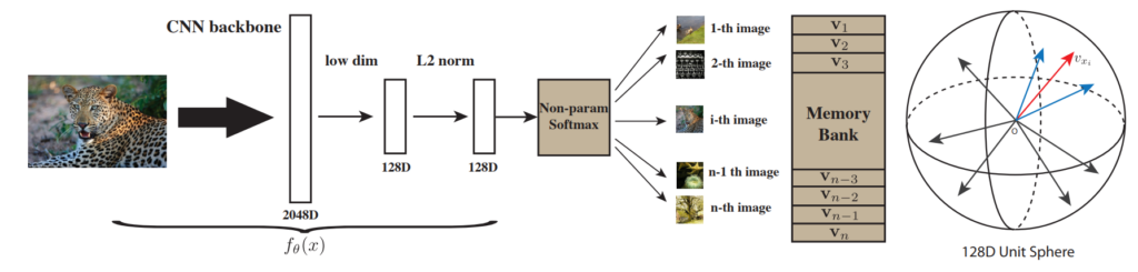
Conceptually this is led up to by the idea of instance discrimination: the work of Wu et al. (2018) scales up the Exemplar-CNN idea ("each image is a separate class") using a memory bank and an NCE-like loss function:
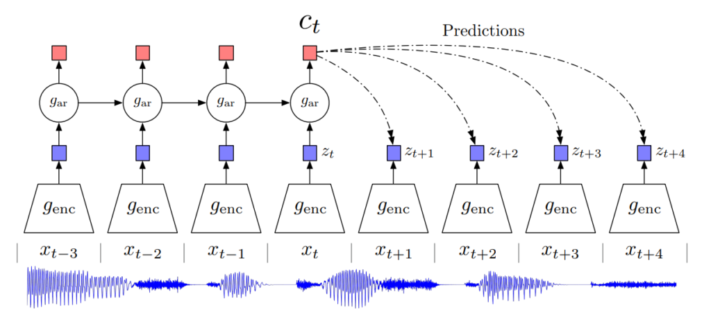
And the closest ancestor of JEPA in this era is Contrastive Predictive Coding, CPC (van den Oord et al., 2018): from the context we predict the latent representation of a future chunk of the signal, optimizing the so-called InfoNCE loss function.
InfoNCE in its canonical form looks like this:
![\[\mathcal{L}_{\text{InfoNCE}} = -\log \frac{\exp\big(\mathrm{sim}(z, z^{+})/\tau\big)}{\sum_{j}\exp\big(\mathrm{sim}(z, z_{j})/\tau\big)},\]](https://cdn.prod.website-files.com/677e6981f4fde5d98559a350/6a579c0bdf275a4310215803_6a5791f730354a60de858d0e_6a5465450379a4151a7a3bb9_quicklatex.com-c20a6f57296e32887fefaf7616d10675_l3.svg)
that is, among a bunch of candidates $z_j$ we have to pick the right positive example z+. Formally this is just multiclass classification. Here's a figure from a paper on audio, but it applies to any modality in exactly the same way:
The name Info-NCE came about because it is both a direct descendant of that same noise-contrastive estimation and, at the same time, a variational lower bound on the mutual information between context and target:
![\[\hat I_{\text{NCE}} = \log N - \mathcal{L}_N \;\le\; I(X;C),\]](https://cdn.prod.website-files.com/677e6981f4fde5d98559a350/6a579c0bdf275a43102157de_6a5791f630354a60de858cfe_6a54658cb6e12e756ccb0023_quicklatex.com-8bd608336debede4713afa00521cfcc1_l3.svg)
where LN is the (non-negative) loss function itself. Since LN is nonnegative, it immediately follows that the mutual information is lower bounded by log N, and this is one of the main difficulties of NCE. If the true mutual information between the views is greater than log N, the bound hits a ceiling and stops giving any useful signal about the "extra" information: no matter how long you train, the estimate won't rise above log N. The only way to raise the ceiling is to increase N, i.e. add more negatives.
There's a simple information-theoretic intuition here, too: a contrastive task is a choice between N options, and with an N-way multiple choice you can, in principle, certify no more than log N nats of dependency.
This is the theoretical explanation of why people always wanted more and more negatives. Hence the race for large batches (SimCLR), memory banks (instance discrimination), and queues (MoCo); let's unpack that a bit.
Consider two important 2020 models that made contrastive self-supervision more practical and, along the way, gifted JEPA a couple of important details. The first is MoCo (He et al., 2020), which views the task as a dictionary lookup: there is a queue of negatives and a momentum encoder of keys, whose weights are an exponential moving average (EMA) of the main encoder.
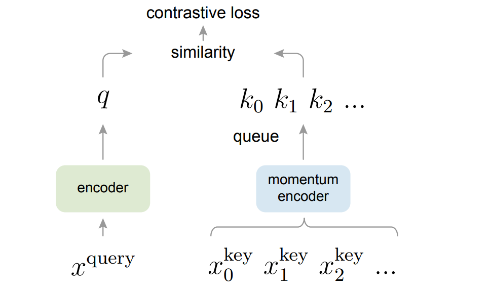
This EMA encoder will become the direct technical ancestor of the target encoder in I-JEPA.
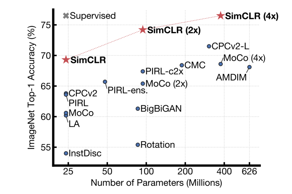
The second important work is SimCLR (Chen et al., 2020), which showed that nothing exotic is needed: an ordinary Siamese network plus InfoNCE, but with large batches, strong augmentations, and a projection head (a small MLP on top of the encoder that you later throw away).

Here it is finally time to spell out how such models are generally compared. The standard protocol is linear probing: we freeze the pretrained encoder and train a single linear classifier on top of it; if the features are good even with such a weak "reader," then the encoder has learned something useful.
So then, SimCLR delivered 76.5% top-1 on ImageNet under this protocol, on par with a ResNet-50 trained with supervision; from that moment self-supervision started entering the mainstream.
Let me note in passing that the very same contrastive approach, but applied to "image / text caption" pairs, gave us CLIP (Radford et al., 2021). Conceptually it was still the same Siamese construction of two views of one object, only the views were an image and its caption:
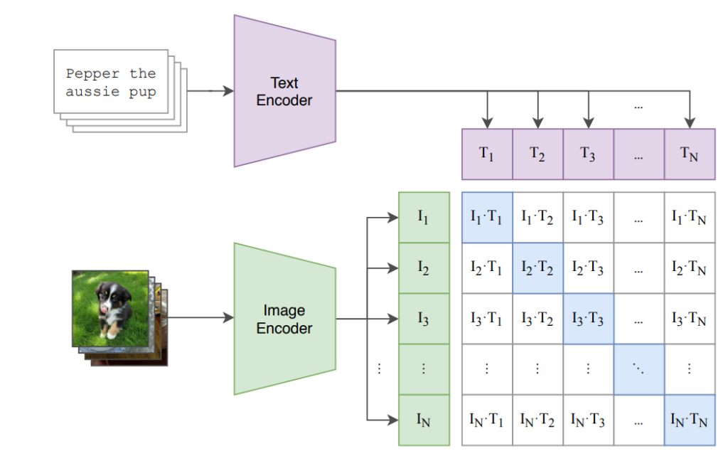
The result was probably the most commercially successful Siamese network in history, and at the same time a bridge between vision and language on which half of today's multimodal systems still stand.
What the contrastive loss actually does was elegantly worked out by Wang, Isola (2020): in the limit, InfoNCE decomposes into two understandable terms, alignment (positive examples placed close together) and uniformity (vectors spread evenly over the sphere).
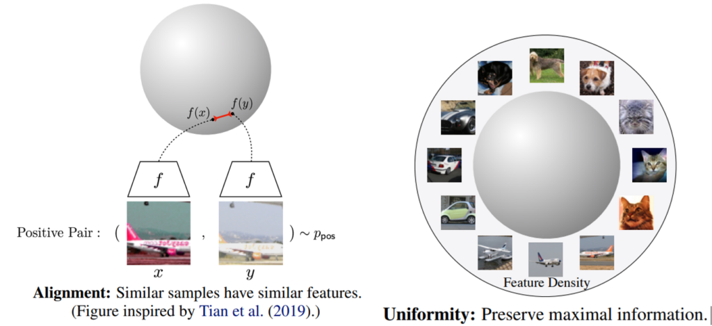
This is an important idea, and we'll come back to it in the theory section. JEPA will inherit the "alignment" part of this story while striving with all its might to shed the dependence on negatives and on aggressive augmentations, because the contrastive approach has a fundamental cost: it needs negative examples, and the higher the dimension, the more of them you need. Hence the main question of the next era: can we get by with no negative examples at all?
It turned out that we can, and JEPA inherits this family directly: all the mechanisms with which JEPA fights collapse were invented here. This is the most important part of our story, so let's take it slowly.
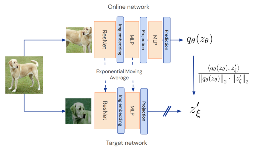
It all started with a rather counterintuitive work: BYOL (Bootstrap Your Own Latent; Grill et al., 2020) learns with no negatives at all and yet does not collapse. The method rests on asymmetry: there's an online network (encoder plus projector plus predictor) and a target network (the same encoder, but with EMA weights from the online one).
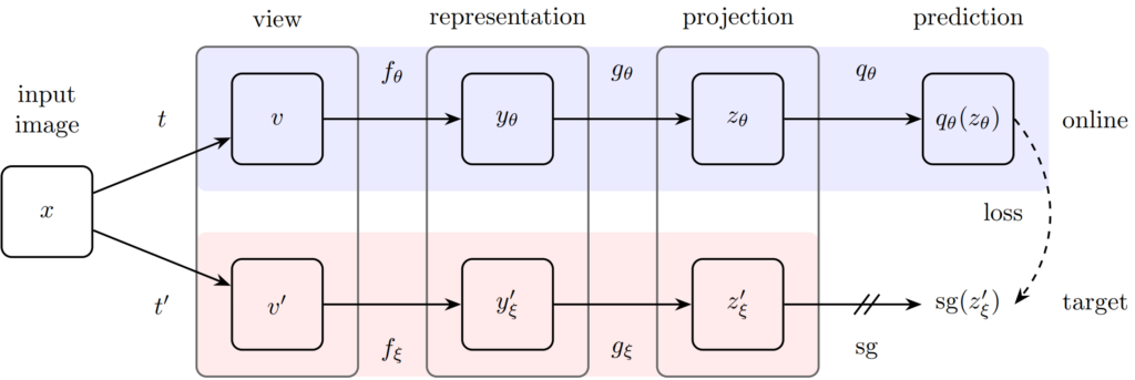
The online network learns to predict the target network's output from a different augmentation of the same image, and there is a stop-gradient on the target. The target, that is the teacher, turns out to be a slowly moving exponential moving average; it always lags a little, and if the "student" is suddenly carried off toward collapse, the teacher still remembers "how things used to be" for a while and keeps the target from collapsing instantly.
Why doesn't BYOL collapse if nothing explicitly pushes the vectors apart? The answer is quite a detective story!
Fairly quickly, enthusiasts discovered that if you remove batch normalization from BYOL, it does collapse, and put forward a beautiful theory: batchnorm smuggles in negatives because normalization forces the embeddings of different images to differ from each other; in this way, batchnorm basically provides repulsion force!.
The theory lived for a few months, until the authors themselves showed (Richemond et al., 2020) that BYOL works perfectly well with no batch statistics at all, using group normalization and weight standardization; batchnorm turned out to be useful for optimization but in no way a secret source of negatives.
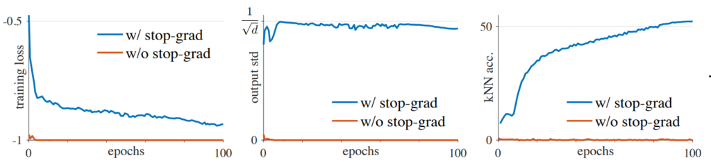
Definitive clarity was brought by SimSiam (Chen & He, 2021) with one careful experiment: you can throw out both EMA and momentum, keep just a predictor on one branch and a stop-gradient on the other, and it turns out this minimal configuration is already enough. It's precisely the stop-gradient that keeps the system from sliding into the trivial fixed point; remove it, and the loss immediately collapses to a constant:
In parallel, a school of thought developed that did unsupervised learning through clustering. SwAV (Caron et al., 2020) predicts, from one view of a picture, the cluster assignment of another view:
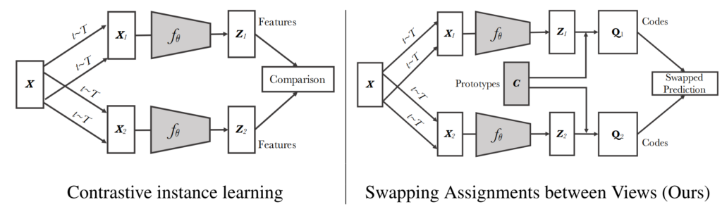
This method avoids collapse by balancing the clusters via optimal transport (the Sinkhorn algorithm): you can't dump all the pictures into one cluster if the clusters are required to be filled evenly. Along the way SwAV introduced multi-crop, the augmentation "two big crops plus several small ones", or simply "two crops at different scales," which almost everyone later adopted. Here's an example from that same BYOL (Grill et al., 2020):
Yet another school fought collapse through explicit regularization of the statistics of the representation itself, with no asymmetry or EMA whatsoever.
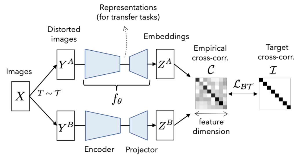
Barlow Twins (Zbontar et al., 2021) pulls the correlation matrix between the embeddings of the two views toward the identity: ones on the diagonal (invariance), zeros off the diagonal (decorrelation, so that coordinates don't duplicate one another). This is exactly Barlow's redundancy-reduction principle that we started with, and hence the method's name.
VICReg (Bardes et al., 2022) does the same thing head-on, with three terms:
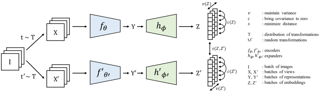
VICReg and Barlow Twins are important for our story because the 2022 manifesto (LeCun, 2022) pointed to these methods as the "correct", regularization-based alternative to EMA tricks. And it's precisely VICReg that was later included into I-JEPA to stabilize training, giving rise to C-JEPA (Mo et al., 2024, a spotlight at NeurIPS), but more on that below.
Finally, there's the distillation school, DINO (Caron et al., 2021): a student network fits its distribution to the output of a momentum teacher, and collapse is averted by centering and sharpening the teacher's distribution. I hope you haven't gotten lost among these model diagrams, which all look roughly the same; but there's a lot of meaning in the small differences here:
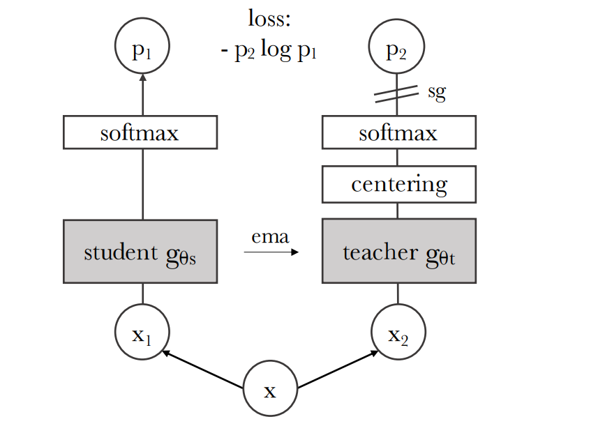
DINO stands for self-distillation with no labels, and it's a direct descendant of the classic knowledge distillation (Hinton et al., 2015), except there's no labeled teacher here; the student distills itself from its own averaged past.
DINO is famous for a side effect: in the attention maps of a ViT, semantic segmentation of objects emerges all by itself.
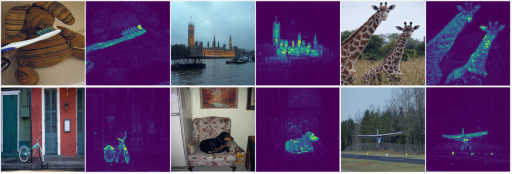
This line of models was continued in DINOv2 (Oquab et al., 2023), which also has iBOT (Zhou et al., 2022)—masked token prediction in a self-distillation regime—inside, and DINOv3 (Siméoni et al., 2025), a 7B model trained on 1.7 billion images, which today is the main "pure-SSL" competitor to JEPA in the quality of visual features.
To wrap up this section, let's summarize. Here are the five mechanisms we've seen, which will recur below in various combinations:
By the end of the post we will add a sixth item to this list, one that tries to replace all these "hacks" with a single rigorous theorem.
While some fought collapse without negatives, others developed a completely different branch of self-supervision: masked image modeling (MIM).
The very idea of "corrupt the input and reconstruct it" is a venerable classic embodied by, e.g., denoising autoencoders (Vincent et al., 2008), and the inpainting from the pretext era was their spatial variant.
The recipe first really took off in NLP: BERT (Devlin et al., 2019) was not an ordinary language model like GPT, but specifically a masked one, and it made MLM (masked language modeling) the main way to learn representations in NLP. Computer vision, naturally, wanted to use such a method too. MIM is BERT for images, and this branch matters to us as an antagonist: JEPA defines itself precisely in opposition to it.
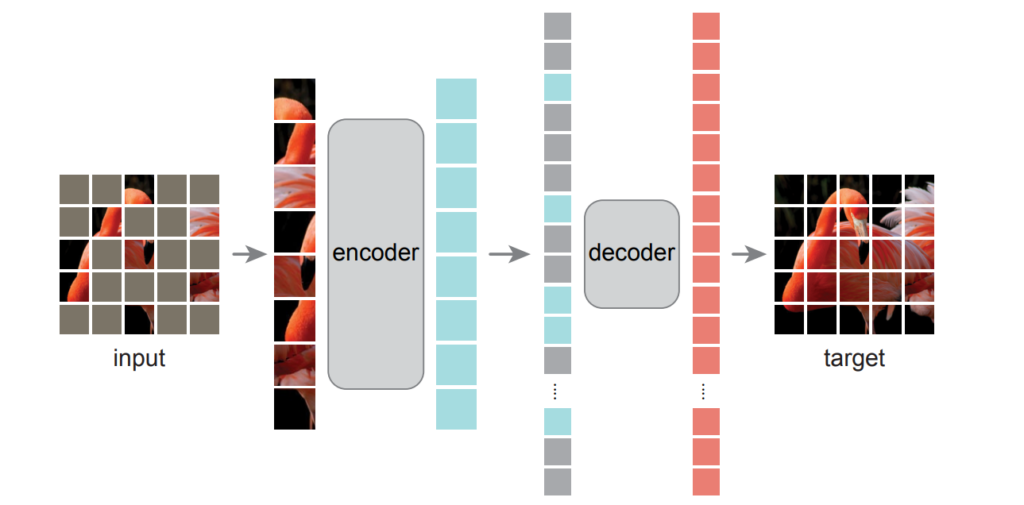
The idea is simple: we hide some patches and ask the model to reconstruct what's hidden. MAE (Masked Autoencoder; He et al., 2022) reconstructs raw pixels under aggressive masking (about 75%) with an asymmetric encoder-decoder; it's the main MIM baseline.
BEiT (Bao et al., 2022) predicts discrete visual tokens. There's also a curious intermediate point — MaskFeat (Wei et al., 2022), which predicts HOG features instead of pixels: no longer the raw signal, but not yet a learned representation either, exactly halfway.
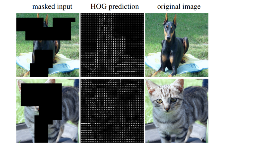
This was a powerful line of models, but JEPA's main objection is directed at it: reconstructing pixels means spending the model's capacity on inherently unpredictable and low-information detail. More on that one chapter from now.
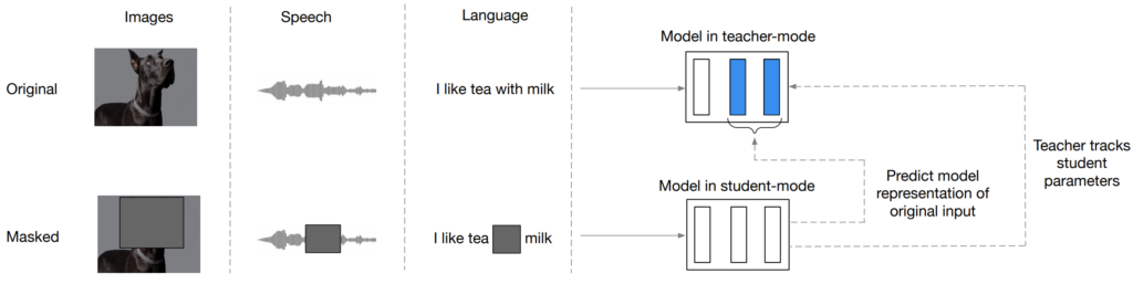
And there were two 2022 works that became the immediate technical precursors of I-JEPA. The first is data2vec (Baevski et al., 2022), which predicts not pixels and not tokens but contextualized latent representations of the full input from a masked view, via an EMA teacher, and does so at once for speech, vision, and text.
The second is Masked Siamese Networks (MSN; Assran et al., 2022), from the same Meta team that would later make I-JEPA: the representation of a masked view is fit to the representation of an unmasked one in a Siamese setup.
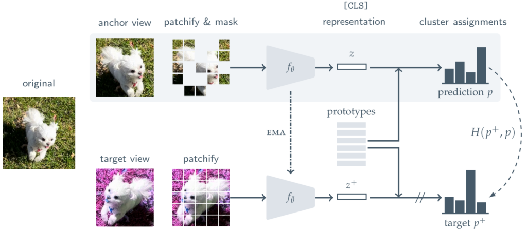
The method here isn't entirely supervision-free, but it uses labels very sparingly — 75.7% on ImageNet with only 1% of labels.
So by the time we reach I-JEPA, it is important to remember that it didn't grow out of thin air: it's a synthesis of a very dense neighborhood — BYOL and SimSiam (asymmetry and EMA), VICReg (regularization), data2vec and MSN (latent targets and masking), CPC (prediction in latent space). What's interesting about I-JEPA is not the idea of latent prediction itself, but what exactly to take from all of this and how to trim away the excess.
Let me note here as well that this whole zoo already runs on transformers (Vaswani et al., 2017) and, in particular, on the Vision Transformer (ViT; Dosovitsky et al., 2020), which slices a picture into patch-based tokens.
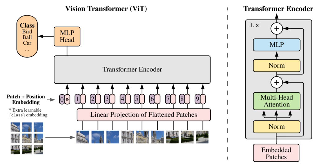
It's precisely ViT that gives us that grid of patches on which it's very convenient to do block masking.

And now we've finally arrived at the JEPA family proper. This idea first appears inside a large program, in the position paper "A Path Towards Autonomous Machine Intelligence" (LeCun, 2022). It's more of a position paper, a manifesto about what an autonomous intelligence should be, with no benchmark numbers or tables, and indeed no specific technical details either.
LeCun's motivation is partly arithmetic, and he likes to recompute it out loud: a four-year-old has been awake for about 16 thousand hours, and over that time roughly 1015 bytes have passed through their optic nerve — tens of times more than all the text on which the largest LLMs are trained. And on that content the child has managed to acquire a mass of very interesting intellectual abilities; here's a picture LeCun often shows on this point:
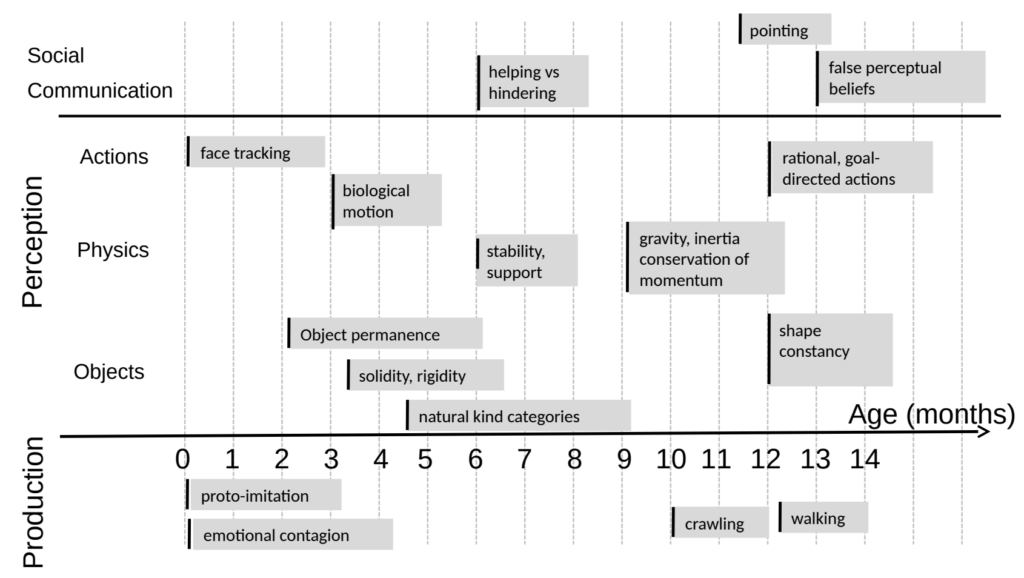
The conclusion from this is that the main source of training data is not text but the sensory stream, and you can learn from it through self-supervision, without any labels. What remains is to figure out what exactly to learn from that stream; the manifesto's answer is world models.
LeCun proposes a modular cognitive architecture, which in the paper he directly overlays onto the brain:
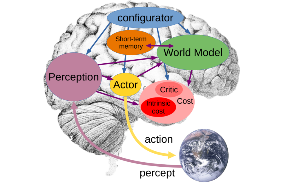
There are six main components here:
LeCun then elaborates on them, and by his design all the modules turn out to be differentiable, so planning reduces to optimizing a sequence of actions with respect to the predicted future cost. LeCun calls this Mode-2 (literally after Kahneman), slow deliberate reasoning. This reasoning can then be "compiled" into a fast reactive policy (Mode-1).
And the world model module in is proposed as a non-generative architecture:
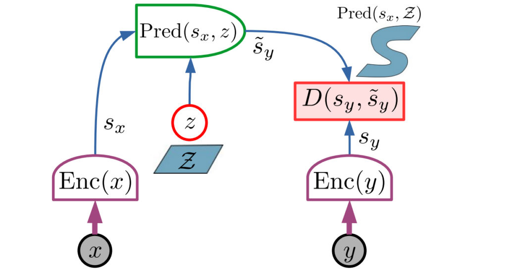
Formally, the general JEPA idea is arranged very much like what we saw above. From a context x and a target y, two encoders build representations:
![\[z_x = f_\theta(x),\quad z_y = f_\xi(y).\]](https://cdn.prod.website-files.com/677e6981f4fde5d98559a350/6a579c0edf275a43102158d3_6a5791f930354a60de858ddb_6a546f6548dc54aff905f3db_quicklatex.com-219687e958ca0052fff226250318a683_l3.svg)
The predictor reconstructs the target from the context and a description c of what is being predicted (position, time offset, action):
![\[\hat z_y = g_\phi(z_x, c).\]](https://cdn.prod.website-files.com/677e6981f4fde5d98559a350/6a579c0edf275a43102158d6_6a5791f930354a60de858dc4_6a546f7d4fabb6487a5d81ed_quicklatex.com-cf17a5ee3adc6813b87bc162c94e3e9a_l3.svg)
Training minimizes the distance between the prediction and the (stop-gradient) representation of the target, plus an optional regularization against collapse:
![\[\mathcal{L}_{\text{JEPA}} = \mathbb{E}_{x,y,c}\, D\big(g_\phi(f_\theta(x), c),\; \operatorname{sg}(f_{\bar\theta}(y))\big) \;+\; \lambda\,\mathcal{R}.\]](https://cdn.prod.website-files.com/677e6981f4fde5d98559a350/6a579c0fdf275a4310215917_6a5791fa30354a60de858e10_6a546f7d4fabb6487a5d820c_quicklatex.com-9275dfee98e45ef10d55792cf21f39ed_l3.svg)
Here fθ can be an EMA teacher, a frozen encoder, or the same encoder with regularization. There's only one important detail that distinguishes JEPA from the classic Siamese scheme: the encoders are not required to use the same weights, and x and y can be built differently.
Here's the same thing as a diagram:
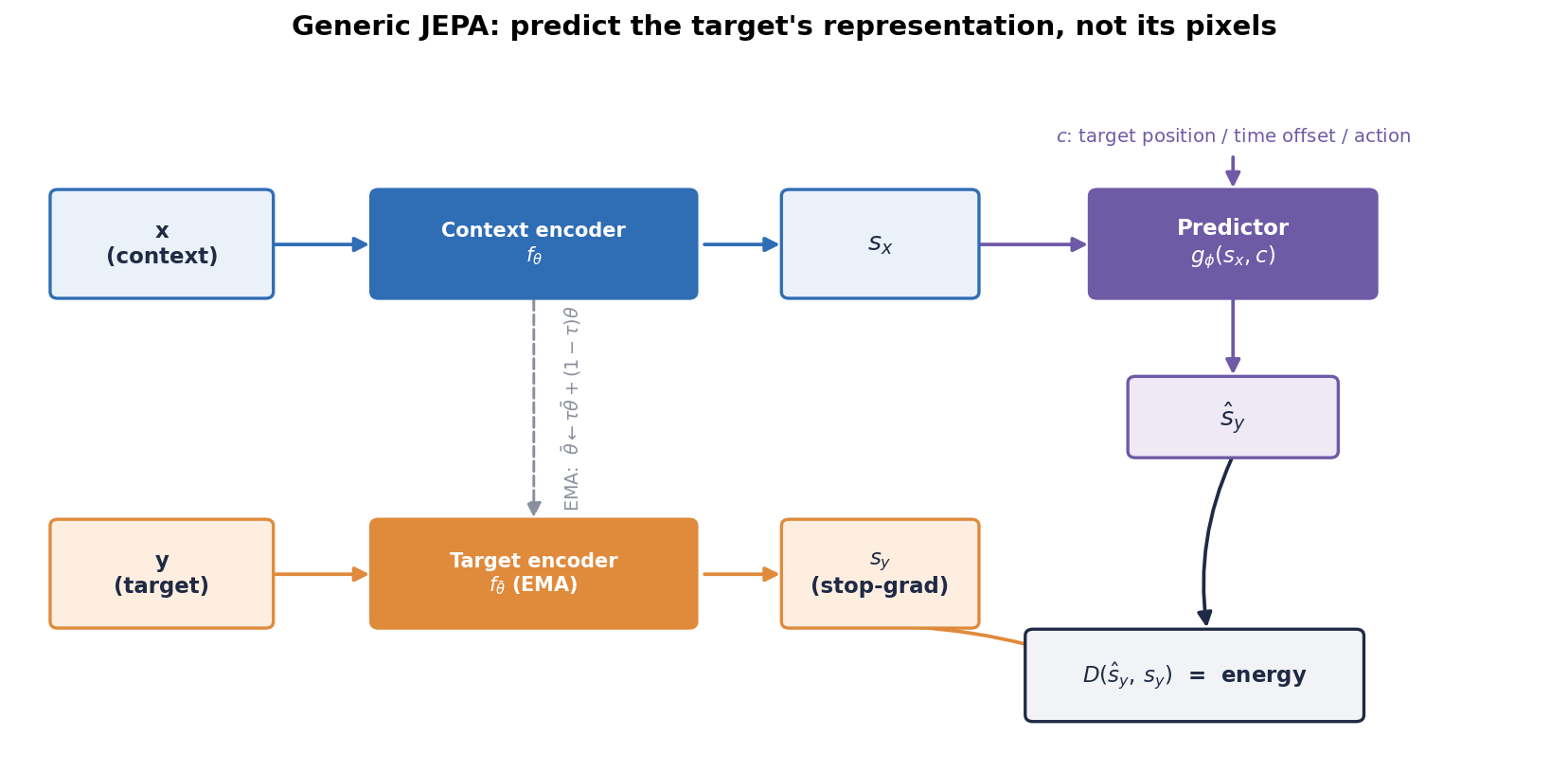
There are two main ideas here; both are not new, but their successful combination is still not so easy to pull off:
The first idea becomes clearer in the energy-based reformulation. Introduce a latent variable z that takes on the part of y that is fundamentally not determined by the context:
![\[E(x,y) = \min_{z}\, D\big(g_\phi(f_\theta(x), z),\; f_\xi(y)\big).\]](https://cdn.prod.website-files.com/677e6981f4fde5d98559a350/6a579c0edf275a43102158f7_6a5791fa30354a60de858df6_6a54f849a6db8869ed595423_quicklatex.com-087477c99ee6eb6edb78fe864f0f2737_l3.svg)
This looks like a small change, but it is very fundamental. The future is multi-valued: a car at a fork can turn left or right, and both branches are plausible. If we build a deterministic predictor with a squared loss, it learns the conditional mean. And if the encoder maps "left" and "right" to two different vectors, then their mean may correspond to no real future at all — it will hang somewhere in between:
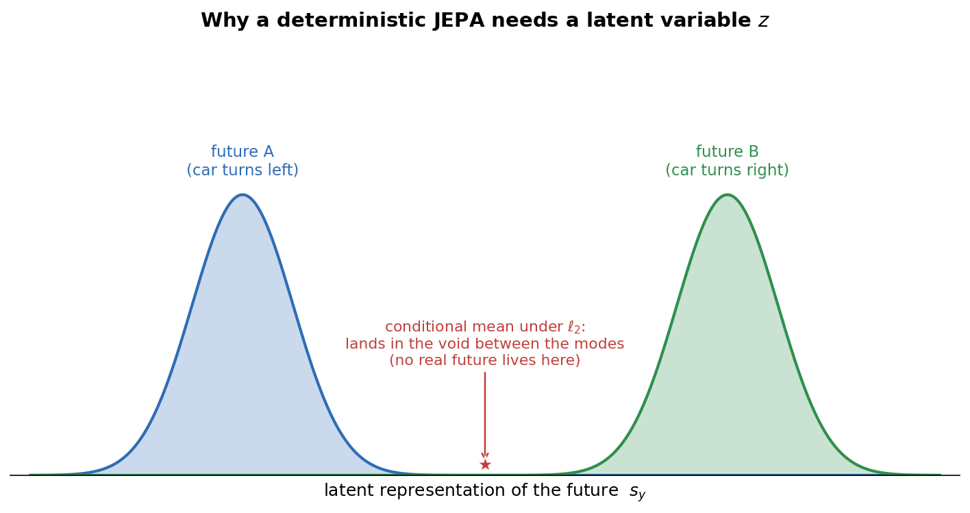
Whereas the latent variable z indexes these alternatives; for each particular value of z you get a plausible variant of the future.
The manifesto spells out four non-contrastive training criteria, each of which has an information-theoretic justification:
Here's how they map onto the general scheme:
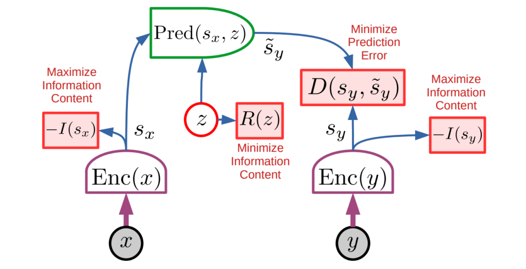
The energy-based lens also splits the anti-collapse methods into two parts: contrastive methods raise the energy of negative examples (and suffer from the curse of dimensionality), while regularization-based ones limit the volume of the low-energy space itself, imposing information constraints on the representations in the spirit of VICReg. JEPA sits entirely in the regularization camp.
Finally, the manifesto also proposes H-JEPA, hierarchical JEPA, where the lower levels predict on short scales and in fine detail, and the upper levels on long scales and in more abstract states.
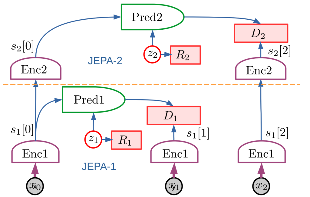
As of 2026 this is still more of a manifesto than a realized system, but H-JEPA remains the conceptual bridge from SSL-on-images to agents that plan.
Now to the second question: why predict representations at all, rather than pixels. This is one of the central points of the whole program. Imagine you're predicting the next frame of a video: a car is driving, and in the background foliage sways and ripples run across a pond. The car's trajectory is useful and predictable; the exact position of each little leaf and each mini-wave is neither.
But a generative model that computes likelihood in pixels is obliged to spend its capacity not only on the car but on the leaves too. JEPA, on the other hand, predicts the representation, and a trained encoder can map a thousand frames with different leaf configurations to nearby vectors, letting the predictor focus on the stable factors. The capacity for reliable abstraction here is not a shortcoming but exactly what we want.
It sounds nice in principle, but there are some caveats:
But with caveats or without, they did in fact make a working model out of the manifesto — and more than one. Let us move on to these models.

I-JEPA (Assran et al., CVPR 2023) is the first clean implementation of the idea for images. The task is stated as follows: from one context block of an image, predict the representations of several target blocks of the same image. Here's the comparison with the standard approaches, and on the right the general JEPA scheme proper:
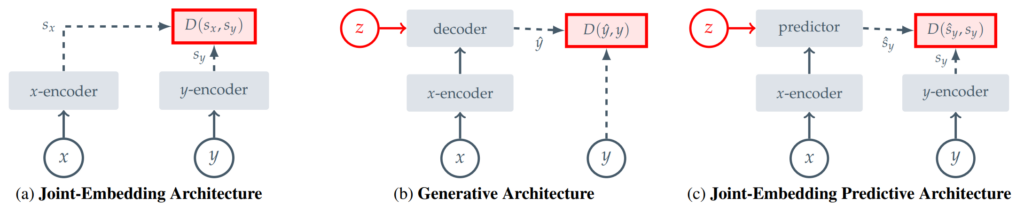
Three networks are at work here:

The loss function is the average L2 distance between the predicted and target representations over M target blocks:
![\[\mathcal{L} = \frac{1}{M}\sum_{i=1}^{M}\sum_{j\in B_i}\big|\hat s_{y_j} - \operatorname{sg}(s_{y_j})\big|_2^2.\]](https://cdn.prod.website-files.com/677e6981f4fde5d98559a350/6a579c0edf275a4310215900_6a5791fa30354a60de858e01_6a5470d7a7e64d5103a20295_quicklatex.com-c1a6d154a7cef29f8804fbe615099666_l3.svg)
As you can see, there are no negative examples here, no pixel decoder, and no contrastive terms in the loss function. Only one mechanism fights collapse here, namely the EMA target with a stop-gradient: the target parameters follow the context encoder as
![\[\bar\theta \leftarrow \tau\bar\theta + (1-\tau)\theta\]](https://cdn.prod.website-files.com/677e6981f4fde5d98559a350/6a579c11df275a43102159b5_6a5791fd30354a60de858ec4_6a5470f2b97359ee7ab78142_quicklatex.com-867af3ecac8770a38afbdfbbac355422_l3.svg)
(the momentum τ starts at 0.996 and grows linearly toward 1). Since the target lags and receives a stop-gradient, the trivial constant solution stops being a fixed point.
Next come three important architectural decisions, in which the main novelty essentially resides. The first is multi-block masking, the very thing that makes the features semantic. We take M=4 target blocks with a random scale in the range (0.15, 0.2) of the area and aspect ratio in (0.75, 1.5), and then one large context block with scale (0.85, 1.0), from which we cut out intersections with the targets.
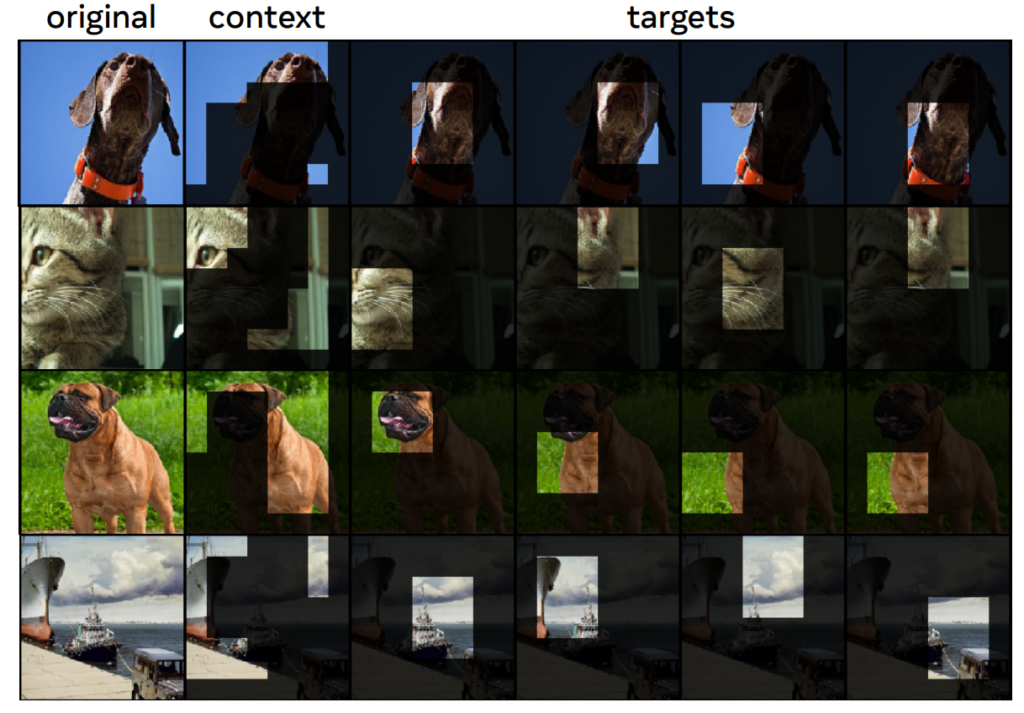
The intuition is that predicting several large, meaningful blocks from an informative but spatially incomplete context means being forced to model object-level structure, their meaning, rather than guessing local texture.
The second decision is masking at the output of the target encoder, not at the input: the targets are cut out of the representations of the full image, not out of raw pixels, so each target patch already "knows" its context (it's been contextualized by a full pass of the encoder), and the targets come out much more semantic.
And the third is efficiency: backbones from ViT-B/16 to ViT-G/16, and importantly, a ViT-H/14 trains on ImageNet in less than 72 hours on 16 A100s; by the standards of today's frontier budgets that's peanuts, but even back then it was several times cheaper than the MIM methods.
It came out especially telling that I-JEPA is strong on low-level spatial tasks like object counting and depth ordering: this means the predictor really does learn spatial structure, and not just global invariance.
So it turns out that I-JEPA absorbed three of the traditions we discussed above:
But so far I-JEPA is not the agent architecture from the manifesto. There are no actions here, no planner, no critic, no long-term memory, no hierarchy, no latent variable for a multi-valued future. It's an application of the JEPA principle to representation learning, and nothing more.
With the move to video, the JEPA idea becomes genuinely ambitious, because video has time, which means there's dynamics, which means a world model has come into view.
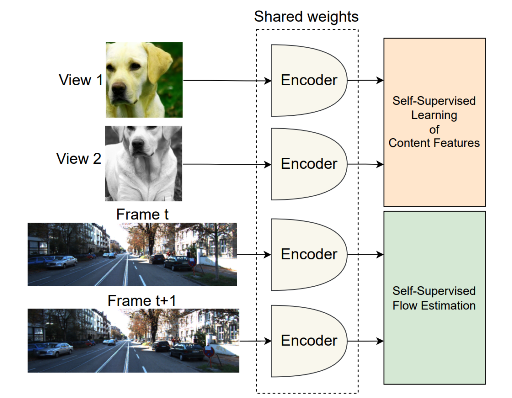
A transitional link here is MC-JEPA (Bardes et al., 2023), which in one encoder learns both content (what's in the scene) and motion (optical flow, how it moves). Ordinary SSL works with content but ignores motion, whereas flow-estimation methods, conversely, model motion without understanding content; MC-JEPA tries to combine them:
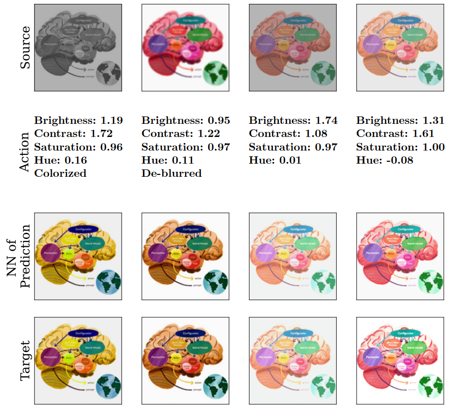
Another conceptually important turn is made by the work on Image World Models, IWM (Garrido et al., 2024). In most SSL the predictor is scaffolding that gets thrown away after training. IWM is based on the following idea: what if the predictor itself is a useful, reusable world model?
The authors generalize the JEPA task from masking to global photometric transformations (predict, in latent code, what will happen if you change the brightness or color) and show that the quality of such a predictor is determined by three levers: conditioning, task difficulty, and the predictor's capacity. Here the predictor stops being garbage and becomes an object of study. In the end IWM really can predict the results of transformations of this kind (NN of prediction is the nearest neighbor from some dataset in representation space, since we are predicting representations):
And training proceeds almost as usual, only now with the new transformations:

And finally, the flagship — V-JEPA, "Revisiting Feature Prediction for Learning Visual Representations from Video" (Bardes et al., 2024). It trains exclusively by feature prediction on about 2 million public videos, with no pretrained image encoder, no text, no negatives, and no pixel reconstruction (the pixel alternative for video is represented by VideoMAE, Tong et al., 2022).
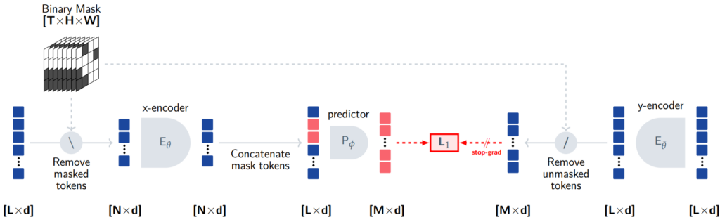
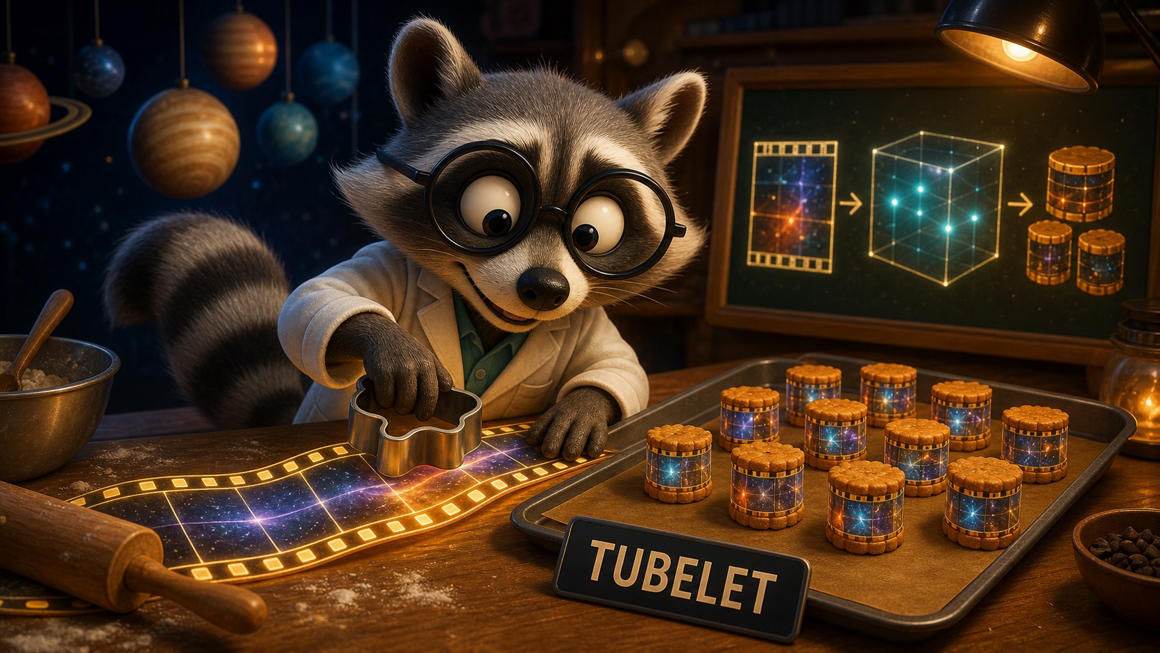
The key trick is aggressive spatiotemporal masking: the video is cut into so-called tubelets, i.e. patches with temporal extent; the masks are stretched across the whole time axis (otherwise temporally adjacent frames almost duplicate each other and the task becomes trivial: the model can simply copy the answer from the neighboring frame); there are short-range masks (a union of 8 blocks, about 15% of the frame) and long-range ones (2 blocks, about 70% of the frame), and on average about 90% is masked; the targets are supplied by an EMA encoder, and the loss function is L1 regression.
The main claim of V-JEPA is not that it predicts the future in full detail as a world model. It's that feature prediction alone yields a frozen representation that transfers both to appearance tasks and to motion tasks.
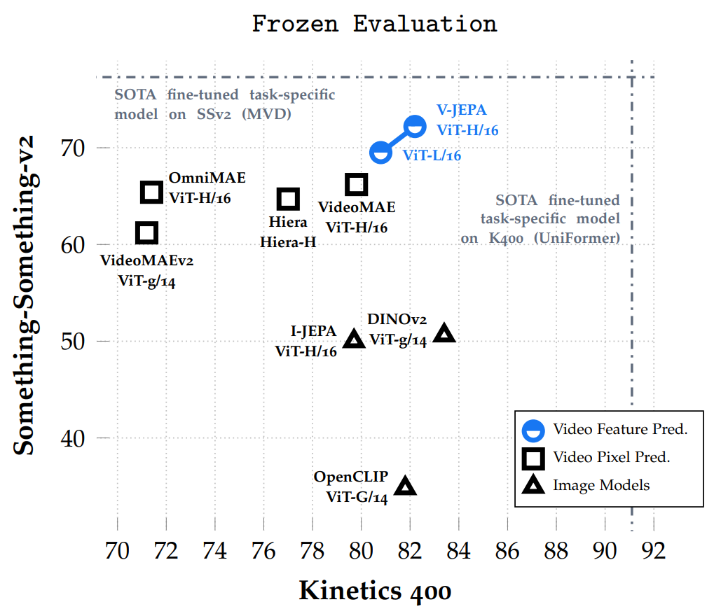
The numbers here, as usual, leave room for criticism—there can be different evaluation protocols, and confusion on this basis is a common thread in the literature—but you can see that latent prediction of the future is closer to predictive coding (CPC) than to autoregressive or diffusion-based video generation.
Here let me recall another beautiful idea from computational neuroscience: slow feature analysis (Wiskott, Sejnowski, 2002). The hypothesis there is this: semantically important quantities change slowly over time (a car drives along its trajectory, objects don't flicker), while sensory noise is fast (each leaf trembles in its own way), so "look for the slow stuff" is by itself a decent principle for unsupervised feature learning.
An early analysis of JEPA world models was titled exactly that: "Joint Embedding Predictive Architectures Focus on Slow Features" (Sobal et al., 2022); it shows that temporal latent prediction naturally pulls out the slow components of the signal. This nicely closes the loop on the intuition about leaves and the car: JEPA is good not because it "ignores details," but because what's slow and predictable in the world almost always coincides with what's meaningful.
And also, when JEPA moved to video, it became appropriate for the first time to ask: does this model understand physics? The work on intuitive physics (Garrido et al., 2025) uses the "violation of expectation" paradigm from developmental psychology: models are shown possible and impossible continuations (an object disappears behind a screen and doesn't come back; it passes through a wall), and we watch whether the model is surprised, that is, whether the prediction error rises on the impossible variant.
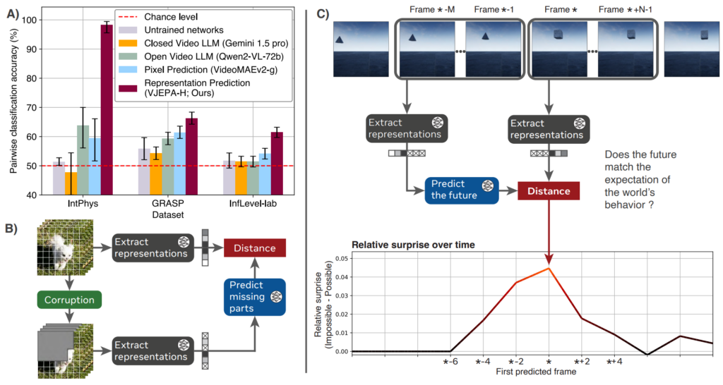
The result came out very positive: predictions in latent space grasp object permanence and shape consistency noticeably better than pixel prediction and multimodal LLMs, which often stay near chance.
This, of course, doesn't prove that JEPA has already learned "common sense" about the surrounding world, and harder benchmarks immediately appeared — IntPhys 2 (Bordes et al., 2025) and Minimal Video Pairs (Krojer et al., 2025) — on which SOTA models are again near chance while humans are near ceiling. But note that this is already a slightly different question: you can now ask models "what exactly is in your representations?", not only "what's your accuracy on this benchmark?".

And now we finally come to the point that all of this was for. V-JEPA 2 (Assran et al., 2025) is not just a scaled-up version of V-JEPA, but a version that finally connects representation learning with a world model for planning, the very thing LeCun's manifesto promised us from the start.
V-JEPA 2 has two training stages and two types of data.
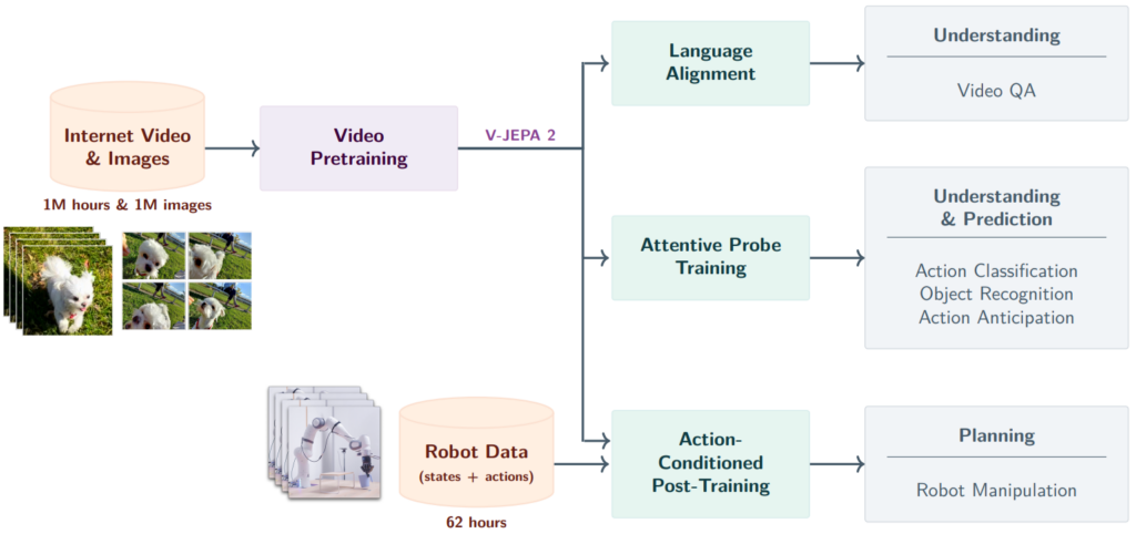
The first stage is pure observation-based pretraining. An action-free encoder (ViT-g, over 1B parameters) is trained on 22 million samples representing over a million hours of internet video plus images, with progressive resolution scaling, 3D-RoPE, and careful data selection. The result is excellent scores on video understanding benchmarks and, tellingly, state of the art on action anticipation in Epic-Kitchens-100, a big jump over specialized models. The authors even tried grafting the frozen encoder onto an 8B LLM (in the LLaVA spirit), and got very strong Video-QA out of it despite the fact that the encoder never saw a single word in its life, and it was answering questions through an "LLM translator". The first stage is on the left in the figure:
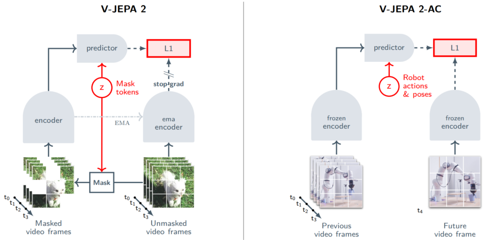
The second stage is V-JEPA 2-AC, a world model with actions (on the right in the figure). The encoder is frozen, and on top of it a predictor of about 300M parameters with block-causal attention is trained; it's trained on less than 62 hours of unlabeled robot-arm video from the DROID dataset, i.e. there's orders of magnitude less data here.
The predictor learns to predict future patch representations from past representations, actions, and the end-effector state. There is a teacher forcing variant and one with long rollouts, but let's not dig into that right now:

Planning then, of course, proceeds directly in latent space. On real robot arms the model works zero-shot: the goal is given as a picture, and model-predictive control by the cross-entropy method (CEM) searches for actions that minimize the L1 distance between the predicted future representation and the representation of the goal; here energy acts as the distance to the goal.
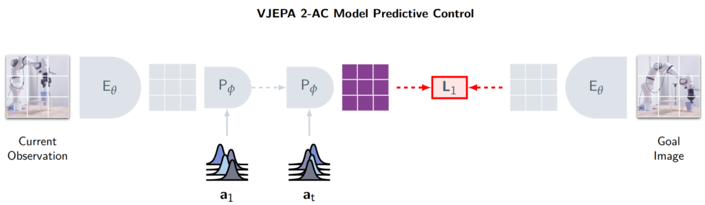
With no data collection from these particular robots, no reward-function engineering, and no task-specific fine-tuning, you get rearranging new objects in a new environment with 65–80% success.
As of today V-JEPA 2 is the clearest realization, closest to the original, of the 2022 promises. But there are obvious limitations: for now it's short-horizon manipulation learning, with given visual subgoals and a separately fine-tuned action model. The full "configurator + actor + critic + memory" stack from the manifesto is still a long way off.

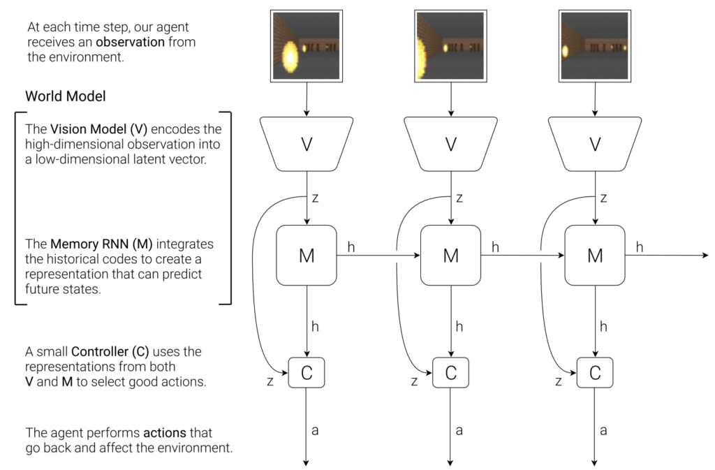
Here it's worth raising our heads a little and looking around, because world models were not invented at Meta. There's a whole tradition of learning an internal model of the dynamics and planning within it. Among the founders here one should count, rather, the work "World Models" (Ha & Schmidhuber, 2018; yes, yes, that same Schmidhuber again!), which trains a VAE plus RNN dynamics, and the controller is trained inside the model's "dream".
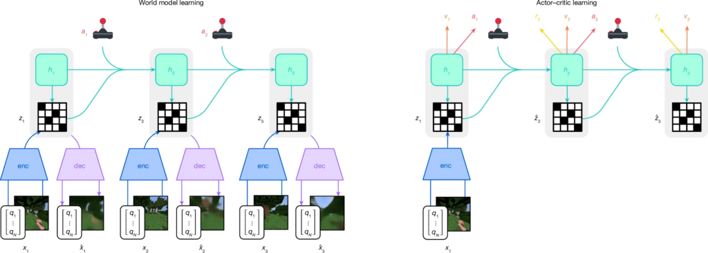
PlaNet (Hafner et al., 2019) trains latent dynamics and plans by that same CEM method in latent space that V-JEPA 2-AC uses. The Dreamer series (Hafner et al., 2020 and onward; DreamerV3, for instance, first came out on arXiv in 2023, and in 2025 also in Nature under the title "Mastering diverse control tasks through world models") trains behavior by "imagination" in latent space:
And finally, we can't but mention MuZero (Schrittwieser et al., 2020), which plans within a learned latent model that in turn predicts only the reward, the value function, and the policy — and never reconstructs observations at all.

There's also a parallel line within reinforcement learning itself. DeepMDP (Gelada et al., 2019) trains a latent model via bisimulation; SPR (Schwarzer et al., 2021) predicts its own future latent states with an EMA target. In essence, this is BYOL transplanted into RL on Atari games, and independently and almost simultaneously at that:

TD-MPC (Hansen et al., 2022) plans in latent space with no decoder; bisimulation metrics (Zhang et al., 2021) build representations that distinguish states only by future rewards.
Here I can recommend a systematic survey by Ni et al. (2024), which brings some order to this whole zoo, in particular analyzing when latent self-prediction in RL is stable and when it collapses. Let me allow myself to copy a table from it, though of course we won't get into all of it right now:
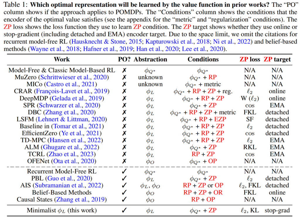
There is, nonetheless, a difference between these directions. Dreamer, PlaNet, and the rest train generative latent dynamics, with reconstruction. MuZero and the whole RL line train value-equivalent models that predict only what's needed to evaluate a move, sothey need a final reward as a signal.
Whereas in JEPA there's a self-supervised latent model without reconstruction, whose sole objective is feature prediction, and training proceeds from passive video, with no rewards or labels whatsoever. Only at the level of V-JEPA 2-AC does this model borrow the planning methods (CEM/MPC) from the Dreamer/PlaNet camp. In other words, the novelty here is not planning in latent space, which was already possible in 2019–2020, but learning purely by passive self-supervision on internet video, with no rewards or reconstruction, yet in such a way that the latent space ends up being fit for planning.
A few more words about the relation with neuroscience, admittedly quite abstract and more inspirational than precise. JEPA fits nicely with the theory of predictive coding (Rao & Ballard, 1999), where feedback connections in the cortex carry predictions of lower-level activity, while feedforward connections carry the error of the prediction.
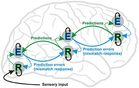
There's also a more general free energy principle in neuroscience, due to Friston (Friston, 2010): the brain minimizes prediction error, a.k.a. variational free energy.
LeCun himself cites predictive coding as motivation, but this is, of course, precisely abstract inspiration, not some claim about modeling the workings of a real brain.
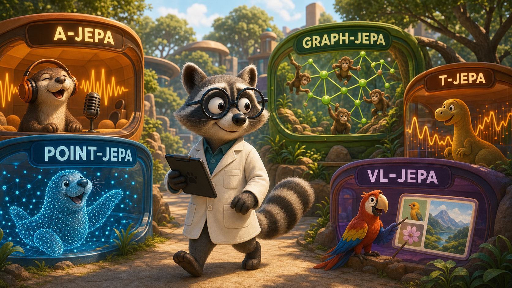
By 2026 JEPA is no longer a single model but a large family united by a common structure: context and target encoders plus a predictor plus masking, EMA or regularization against collapse, and a regression loss in latent space. Let me list a few works, though the list here will of course be inherently incomplete, and new models appear literally every month.
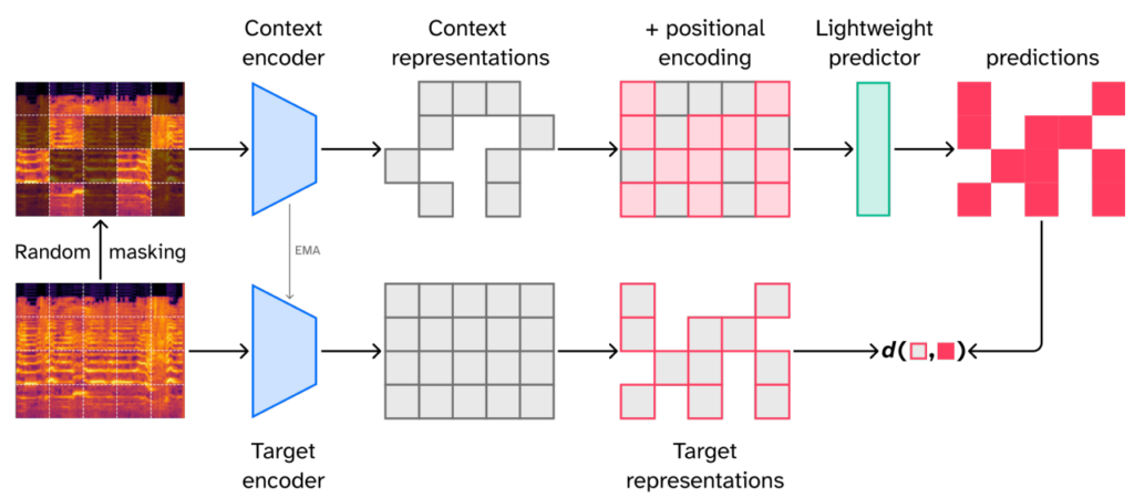
For audio there's A-JEPA (Fei et al., 2023) with masking of mel-spectrograms, and Audio-JEPA (Tuncay et al., 2025); a curious empirical fact is that for audio, random masking beats the vision-style block masking.
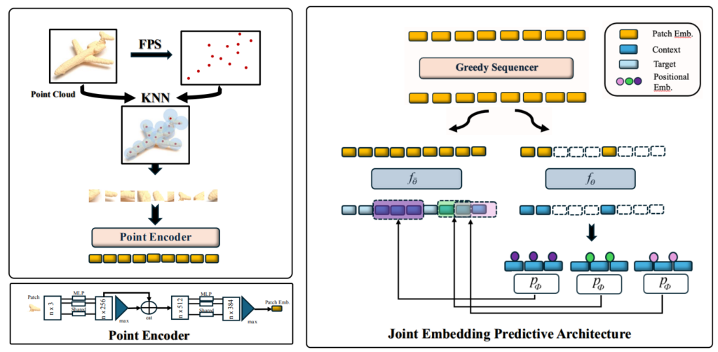
For 3D and point clouds there's Point-JEPA (Saito et al., 2024), where a special sequencer orders the unordered points so that you can take adjacent context/target blocks without reconstructing the input.
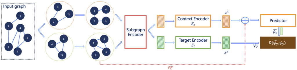
For graphs there's Graph-JEPA (Skenderi et al., 2023), which predicts embeddings of subgraphs, optionally in hyperbolic space, in order to encode hierarchy.
For the brain and biosignals there's S-JEPA for EEG/BCI (Guetschel et al., 2024) and beyond — ECG, fMRI, and so on. For robotics and action policies there's ACT-JEPA (Vujinović et al., 2025), which predicts "chunks" of actions and abstract observations in latent space for imitation learning. The letter T, by the way, has already been independently claimed twice: T-JEPA is both about motion trajectories (Li et al., 2024) and about tabular data (Thimonier et al., 2024); free letters in the alphabet are getting scarcer and scarcer. There are also hybrids with generative models like D-JEPA (Chen et al., 2024), which crosses latent next-token prediction with diffusion and flow matching.
Another model worth a separate mention is VL-JEPA (Chen et al., 2025), an attempt to carry the basic principle over to language. Instead of autoregressive token generation it predicts continuous embeddings of the target texts, and a lightweight decoder is invoked only when the text really has to be "materialized". The motivation here is exactly like that of visual JEPA: many strings express one and the same meaning, so word-by-word likelihood spends capacity on surface form, whereas predicting a semantic embedding collapses paraphrases into a common target.
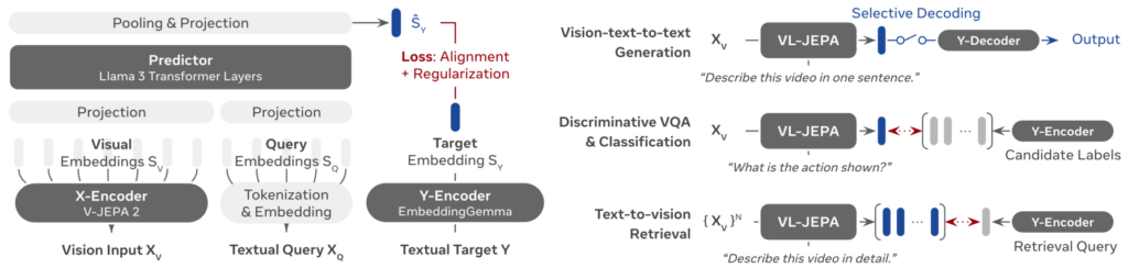
But in language, the form itself is sometimes the task: sometimes you need to recall a quote, an exact name, code syntax, a quantifier's scope. So VL-JEPA, of course, is not trying to say that token prediction is completely obsolete; it offers a kind of "alternative interface", and most likely the future here will belong to hybrid approaches (continuous latent prediction plus selective decoding).
Practice, as often happens in deep learning, runs far ahead of understanding here. But there are some results all the same; let's look at three main directions: what the contrastive methods optimize, why the methods without negatives don't collapse to a constant, and what in all this is specific to JEPA. This section can be skipped if you like, and I won't be going into the mathematical details here, only stating the main results. Also, while we're at it, let me recommend a detailed introduction to the topic: "A Cookbook of Self-Supervised Learning" (Balestriero et al., 2023).
We've already met the work of Wang & Isola (2020) above. They showed that in the limit, InfoNCE decomposes into two parts: alignment that pulls positive pairs together and uniformity that spreads the features over the hypersphere as evenly as possible. What's interesting here is that these two metrics can be optimized directly, with no InfoNCE at all, and you get exactly the same quality. That is, "repelling negatives" is not an end in itself but merely a means of ensuring uniformity; it's precisely uniformity that keeps the representation from collapsing, and alignment that makes it useful. JEPA, as we have seen above, keeps alignment for itself and looks for other, non-contrastive ways to ensure "uniformity" (i.e. to avoid collapse).
The work of Balestriero & LeCun (2022) showed that SimCLR, VICReg, and Barlow Twins, under certain choices of hyperparameters, recover the classical spectral methods: Laplacian Eigenmaps, ISOMAP, Multidimensional Scaling, and others. In the same direction goes the spectral contrastive loss (HaoChen et al., 2021): contrastive learning turns out to be a spectral decomposition of the augmentation graph — a huge graph in which images are joined by an edge if they could have been produced from each other by augmentations — and with provable quality guarantees on downstream tasks at that.
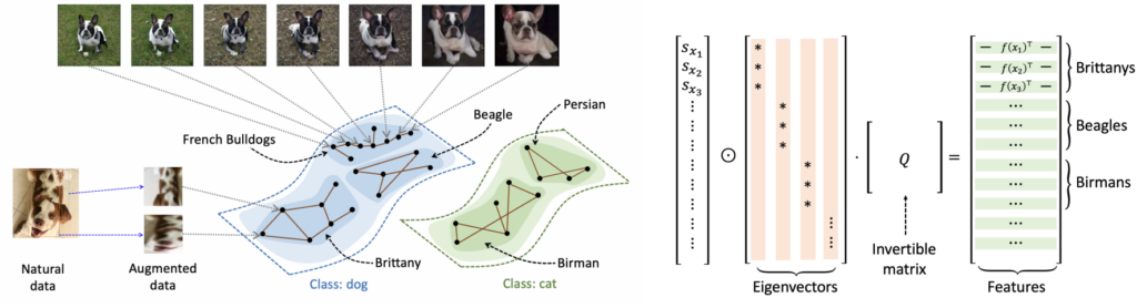
And the work on duality (Garrido et al., 2023) connects contrastive and non-contrastive methods through a spectral and covariance lens and shows that in many ways these are two views of one and the same object.
In other words, the whole zoo of self-supervised learning methods can be regarded as one and the same idea: building a geometry consistent with the augmentation graph. And the differences between methods reduce to *how exactly* we teach our networks that geometry.
Here, to be honest, there is still no single generally accepted explanation, and that in itself is curious.
There's an analysis of the training dynamics of BYOL and SimSiam (Tian et al., 2021): the authors show that the bundle "predictor plus stop-gradient plus EMA" works thanks to a separation of time scales between the predictor and the target and an implicit regularization of the variance, and they even derive from this analysis a simplified method, DirectPred, which sets the predictor analytically.
There is a separate thread about dimensional collapse (Jing et al., 2022): a representation may not shrink to a point, but still "fall through" into a subspace of lower dimension than it has available.
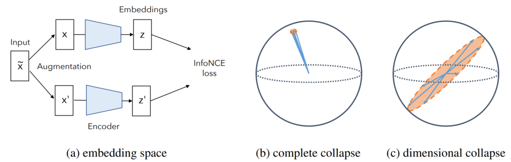
This is a subtler picture than full collapse, and it's precisely what motivates decorrelation methods like Barlow Twins. The degree of such partial collapse, by the way, can be monitored via the effective rank of the representations: the RankMe metric (Garrido et al., 2023) predicts downstream quality quite well with no labels at all.
It's also telling that the EMA target alone turns out to be not a fully reliable safeguard. The already-mentioned C-JEPA (Mo et al., 2024) explicitly notes that in I-JEPA the EMA by itself is not enough to guarantee avoiding collapse, and adds to it the variance and covariance terms from VICReg, after which training becomes more stable and converges faster. So for now JEPA models still rest largely on heuristics rather than on the consequences of some single theorem.
The nicest of the JEPA-specific results is about implicit bias. Littwin et al. (2024) show that in deep linear models JEPA is biased in favor of "influential" features (those with large coefficients) and suppresses noisy high-variance directions, and this bias strengthens with depth. Reconstruction methods like MAE have no such advantage: the pixel target forces them to spend capacity on the noise too. This is exactly the analysis of the idea of why latent prediction can be better than pixel reconstruction not empirically but fundamentally.
It's useful to look at the same thing from an information-theoretic standpoint. Training makes Z = f(Y) predictable from the context X, which means the encoder is rewarded for keeping the components of Y with high conditional predictability and can discard the high-entropy remainder. This relates JEPA to efficient coding, the information bottleneck, and sufficient statistics — and, via the slow features discussed above, to temporal coherence as well.
But there's an important conceptual risk here: does "predictable" coincide with "semantically important" or "important for the task at hand"? Obviously, far from always! A static background can be perfectly predictable yet utterly useless; a rare event can be almost unpredictable yet critically important. For the abstraction to form "in the right direction", you probably also need actions, cost, novelty, hierarchy, and task-conditioning, not passive prediction alone.
And separately adjacent to this is the conditional mean trap we have already discussed: a deterministic predictor under a squared loss averages mutually exclusive futures into a nonexistent mean, so a real stochastic world model absolutely must have latent variables.
The theoretical pinnacle of this line was LeJEPA (yes, that's what the French named it, Balestriero & LeCun, 2025). Its thesis is that, as we've already discussed, the line of JEPA models has all along relied on recipes and heuristics — EMA teachers, stop-gradient, architectural asymmetry, momentum schedules. And one would like, after all, to build a single theory of what distribution of embeddings we even need.
LeJEPA offers two ideas for this. First, the authors prove that an isotropic Gaussian distribution of embeddings is optimal for minimizing the downstream prediction risk over unknown-in-advance tasks. Second, they introduce SIGReg (Sketched Isotropic Gaussian Regularization), a way to force the embeddings to be exactly such Gaussians, by matching their one-dimensional random projections to Gaussians (this is a test in the spirit of Cramér–Wold and characteristic functions) in linear time and memory.
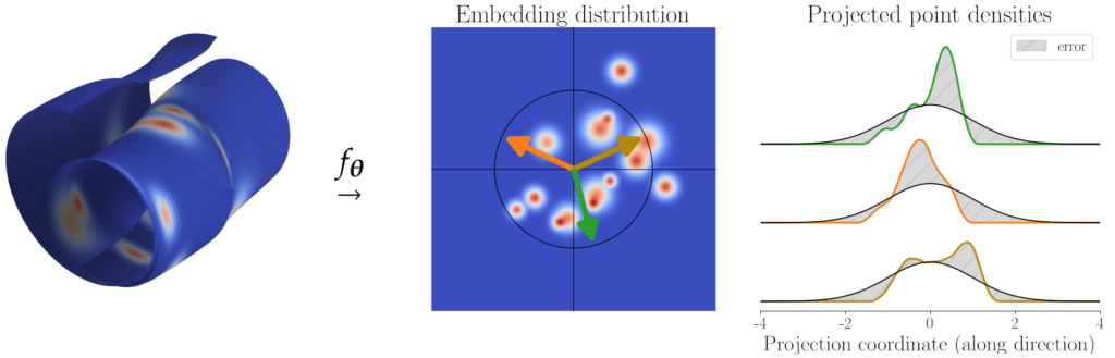
The payoff is that the entire stack of obscure heuristics disappears. No stop-gradient, no EMA teachers, no predictor asymmetry, no manual schedules; the training core fits in about 50 lines and trains stably with a single hyperparameter. Remember the list from the section on methods without negatives? Here's the promised sixth item:
But the topic is far from closed: isotropy was immediately contested. UR-JEPA (Le, 2026), an independent single-author work, not from Meta and not from LeCun (despite the "Le"), notes that a full-dimensional isotropic Gaussian contradicts the manifold hypothesis, according to which embeddings should concentrate on a low-dimensional submanifold rather than fill the whole ball.
Instead of a Gaussian, UR-JEPA aims for a uniformly n-rectifiable measure, and its global PCA spectrum drops by 4–5 orders of magnitude, whereas LeJEPA's is almost flat. So the question of what geometry the embedding space should have remains, for now, an open research topic.
Worth mentioning too is LeWorldModel (Maes et al., 2026); the authors include the same LeCun and Balestriero), where the same philosophy is applied to latent dynamics for control: training proceeds end-to-end directly from pixels with two terms (next-embedding prediction plus a Gaussian SIGReg regularization), and the number of tunable loss hyperparameters drops from six to one.
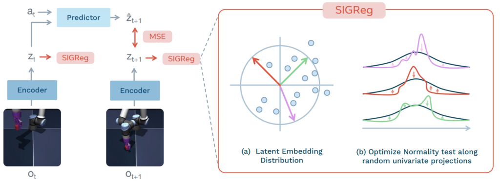
The model here is tiny by today's standards (about 15M parameters), trains on a single GPU in hours, plans tens of times faster than models built on top of large frozen encoders, and physical quantities can be read out of its latent codes.
And the probabilistic branch with latent variables is being developed, for instance, by variational V-JEPA (Huang, 2026), which gives collapse guarantees via the ELBO and a connection to predictive state representations and Bayesian filtering.
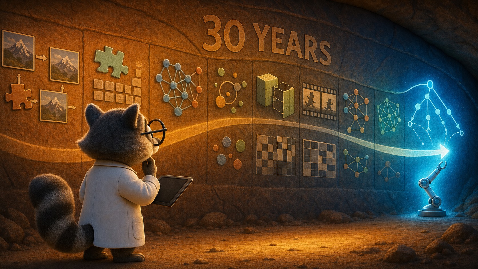
Let me now try to summarize the whole picture. JEPA is the point where LeCun's long-standing energy-based view of learning meets the modern self-supervised toolkit, and where the Siamese-contrastive tradition reappears not in the form "make two views coincide" but in the form "learn abstract states that make the world predictable enough to understand it, imagine it, and plan".
This whole science grows out of Siamese networks, which began back in 1992–1993, and out of contrastive learning, which came at least from the mid-2000s. But it was only in 2022 that LeCun assembled all of it into a single coherent picture and called for predicting meaning rather than pixels. After that, development went much faster: from I-JEPA for images in 2023 to V-JEPA 2, which controlled a robot arm in an unfamiliar lab by planning directly in latent space, only two years passed.
Did LeCun's bet against LLMs win? It does not seem like it at the time. For now JEPA is "merely" one strong and efficient family of self-supervised learning without reconstruction among several (along with self-distillation in the DINOv3 spirit and reconstruction in the MAE spirit), one that stands out for its explicit world-model framing and its excellent compatibility with planning. A full hierarchical H-JEPA with a long horizon, with latent variables for a multi-valued future, and with integrated actor, critic, and memory, still remains a plan for the future.
But the basic thesis is interesting all the same: intelligence needs representations tailored for predicting the controllable and stable structure of the world, rather than for reproducing every observed pixel or symbol. And this thesis, over thirty years, has not just failed to break, it has only accrued ever more convincing implementations. So even if the JEPA family specifically fails to overtake "ordinary" language models, LeCun's bet on "predicting meaning, not pixels" has already changed the way we think about representation learning.
The evolution of data centers towards power efficiency and sustainability is not just a trend but a necessity. By adopting green energy, energy-efficient hardware, and AI technologies, data centers can drastically reduce their energy consumption and environmental impact. As leaders in this field, we are committed to helping our clients achieve these goals, ensuring a sustainable future for the industry.
For more information on how we can help your data center become more energy-efficient and sustainable, contact us today. Our experts are ready to assist you in making the transition towards a greener future.
© 2024 theMind Inc. All rights reserved.


.svg)
.svg)